Policy Optimization with Monotonic Improvement Guarantee

This article is about the theoretical derivation of Policy Improvement Bound and practical policy optimization algorithms discussed in the paper Trust Region Policy Optimization (Schulman, et al, 2015). TRPO is an interesting idea which optimizes policies with guaranteed monotonic improvement. In theory, its algorithm design looks elegant and justified. In practice, it performs robustly on a wide variety of tasks. However, the original proof in Appendix A of their ICML version of paper is a little bit unsatisfying. I will also try to perfect their proof in this article.

• MDPs, Policies, and Optimization
• Analysis on Policy Difference Equation
• Conservative Policy Iteration
• General Policy Improvement Bound
• Trust Region Policy Optimization

Let’s start with some background.

MDPs, Policies, and Optimization

MDPs The interaction between the agent and the environment is typically formulated as an infinite-horizon discounted Markov decision process (MDP), which is defined by the tuple \(\mathcal M = \langle \mathcal S, \mathcal A, \mathcal P, c, \rho_0, \gamma \rangle\). Here, \(\mathcal S\) and \(\mathcal A\) are finite sets of states and actions respectively. And \(\mathcal P\) is the probabilistic transition model, which means when the agent is at some state \(s_t = s\) and it takes an action \(a_t = a\), the probability of the agent moving to a certain subsequent state \(s_{t+1} = s'\) is given by \(\mathcal P(s’|s,a) = \mathsf{Pr}[s_{t+1} = s’|s_t = s, a_t = a]\), where states \(s, s' \in \mathcal S\) and action \(a \in \mathcal A\). The function \(c: \mathcal S \times \mathcal A \rightarrow \mathbb R\) in the tuple is called the expected immediate cost function, indicating how costly it is for a particular move from a particular state. The initial state probability distribution \(\rho_0: \mathcal S \rightarrow \mathbb R\) gives a probability distribution over states \(s_0 \in S\) the agent initially stays. The scalar \(\gamma \in [0,1)\) is the discount factor, which represents the difference in importance between future effects and present effects.

Policies Let \(\Pi\) be the set of all stationary stochastic policies depicting how the agent takes actions in \(\mathcal A\) given states in \(\mathcal S\), i.e., \(\pi(a|s) = \mathsf{Pr}[a_t=a|s_t=s]\) for some \(\pi \in \Pi\). Then for the agent who acts under a certain policy \(\pi\), there would be many possible trajectories of alternate states and actions, like \(\tau = (s_0, a_0, s_1, a_1, s_2 \dots)\), where \(s_0 \sim \rho_0(\cdot), a_t\sim \pi(\cdot|s_t)\) and \(s_{t+1}\sim \mathcal P(\cdot\)|\(s_t, a_t)\). We simply write the trajectory \(\tau \sim \pi\) (sampled by a policy) given context \(\mathcal M\) for convenience. For survival in the environment, or for expanding its individual utility out of individual rationality, the agent always wants to make its cost lower. Thus, the ability to search for an optimal policy \(\pi^\star\) which minimizes the agent’s expected discounted cumulative cost \[\pi^\star \in \arg\min_{\pi \in \Pi} \mathbb E_{\tau\sim\pi} \left[ \sum_{t=0}^{\infty} \gamma^{t}c(s_t,a_t) \right],\]
is a key feature of intelligent agents. The existence and characterization of such \(\pi^\star\) have been widely studied in the theory of optimal control. In reinforcement learning, we are concerned with how to learn or approximate the optimal policy.

Example (2D Navigation Problem as MDP)
The illustration above shows a 2D navigation problem, where Tony plans to go back school \(🏫\) as soon as possible, but unfortunately a volcano \(🌋\) blocks his way. Even worse, a strong east wind \(🌪️\)blows occasionally, which might shift Tony out of the direction intending to move in. To reach out the school in safety, Tony needs to make a detour.
Obviously, Tony is the agent and the map is the environment. The state space consists of all locations in the map, \(\mathcal S = \{(x,y)|x,y\in\{0,1,2\}\}\). The action space contains moves in four directions, \(\mathcal A = \{e_x, e_y, -e_x, -e_y\}\), where \(e\) denotes the unit vector. The trainsition model \(\mathcal P(s'|s, a) = \sum_{s''\in S}\mathtt{move}(s''|s, a) \cdot \mathtt{wind}(s'|s''),\) where \(\mathtt{move}\) is a deterministic model, which assigns a valid move \((s,a,s'')\) with probability 1, and \(\mathtt{wind}\) transports Tony to the location one step left (if valid) with probability 1. Every step causes one unit time cost. Dropping in to the volcano cost an addtional 10 units time penalty.

States Space \(\mathcal S\)	Actions Space \(\mathcal A\)	Trasition Model \(\mathcal P\)	Policy \(\pi\)
\(\{(x,y)\mid x,y\in\{0,1,2\}\}\)	\(\{e_x, e_y, -e_x, -e_y\}\)	\(\mathcal P = \sum\mathtt{move}\cdot\mathtt{wind}\)	such as some deterministic policies.
Cost Funciton \(c(s,a)\)	Initialization \(\rho_0\)	Discount Factor \(\gamma\)	Trajectory \(\tau\)
\(1 + 10\cdot \mathcal P(🌋\mid s,a)\)	\(\rho_0\)-almost surely \(s_0 = (0,0)\)	0.99	e.g., the one shown in illustration

[Terminal] In this problem Tony’s trave has a terminal (school \(🏫\)), while MDP is often in potentially infinit horizon, i.e. non-terminating process. However, we can covert the terminate state to a trap by enforcing the trainsition probability \(\mathcal P(🏫|🏫,\cdot) = 1\), and setting the cost after arrival as 0. [Reward/Cost] Most people write MDPs in maximizing reward other than minimizing cost. Actually, these two are equivelent, by seeing the cost as the negtive reward. If the immediate reward is defined as \(R_a(s,s')\), in our definition, the expected immediate cost is \(c(s,a) = \mathbb E_{s'\sim \mathcal P(\cdot|s,a)} [-R_{a}(s,s')]\), which will be sufficient for policy evaluation and optimization.

Optimization There are roughly there categories of policy optimization algorithms.

• Policy iteration methods, which alternate between estimating the value function and improving policy greedily. Here, the value function \(V^{\pi}:\mathcal S \rightarrow \mathbb R\) is defined as \(V^{\pi}(s)=\mathbb E_{\tau\sim\pi|s_0=s}\left[ \sum_{t=0}^{\infty} \gamma^{t}c(s_t,a_t) \right]\), meaning the discounted expected cumulative cost performing the policy \(\pi\) staring at a specific state \(s\). Once \(V^\pi\) is estimated, we can greedily update policy accordingly. Optimal policies can also be implicitly obtained (though it requires more iterations) by Value Iteration according to Bellman optimality equation: \[V^{\pi^\star}(s) = \min_{a\in\mathcal A}c(s,a)+\gamma\mathbb E_{s’\sim\mathcal P(\cdot|s,a)}\left[V^{\pi^\star}(s’)\right]\] which can be applied to the Q value function \(Q^{\pi}(s,a)=\mathbb E_{\tau\sim\pi|\substack{s_0=s\\a_0=a}}\left[ \sum_{t=0}^{\infty} \gamma^{t}c(s_t,a_t)\right]\).
  In the model-free control problem, policy iteration methods is the foundation of some famous RL algorithms such as Sarsa and Q-learning.

• Policy gradient methods, which parameterize the policy and estimate the gradient of the expected discounted cumulative cost from sampled trajectories. Take the advantage actor-critic method as example, the gradient of loss function is \[\nabla_\theta J(\theta) = \mathbb E_{\tau\sim\pi_\theta} \left[\nabla_\theta \log\pi_\theta(a|s)~A^{\pi_\theta}(s, a)\right], \] where \(A^{\pi_\theta}(s,a) = Q^{\pi_\theta}(s,a) - V^{\pi_\theta}(s)\) is called advantage function, which is useful to reduce the variance while training. Update \(\theta \leftarrow \theta - \alpha \nabla_\theta J(\theta)\) with a suitable learning rate \(\alpha\) each time after estimating advantage function by several steps sampling.

• Derivative-free stochastic optimization methods, such as the cross-entropy method (CEM), which treat the total cost as a black box function to be minimized in terms of the policy parameters. This kind of approaches achieves good results while being simple to understand and implement. However, it relies on deliberately designed hand-engineered policy classes with low-dimensional parameterizations, which is highly task-specific and also limits the expression power of policy models.

On the other hand, gradient-based optimization algorithms can optimize large nonlinear policies such as neural networks so that have much better complexity guarantees. If an efficient training process could also be guaranteed, then the agent would be able to learn more complex and powerful policies.

Analysis on Policy Difference Equation

Let \(\eta(\pi) = \mathbb E_{\tau\sim\pi} \left[ \sum_{t=0}^{\infty} \gamma^{t}c(s_t,a_t) \right]\) denote the expected cumulative discounted cost of policy \(\pi\) for short. A useful identity is given by Kakade & Langford (2002) to express the cost of another policy \(\widetilde \pi\) in term of \(\pi\).

Lemma 1. Given two policy \(\widetilde \pi\) and \(\pi\) for an MDP \(\mathcal M = \langle \mathcal S, \mathcal A, \mathcal P, c, \rho_0, \gamma \rangle\), we have \[ \eta(\widetilde \pi) = \eta(\pi) + \mathbb E_{\tau \sim \widetilde \pi}\left[\sum_{t = 0}^{\infty} \gamma^{t} A^{\pi}(s_t, a_t)\right]
\] where all the notations are defined as above.

Proof. It is easy to see by definition that the advantage can be rewritten as

Therefore the expectation of the advantage \(A^{\pi}\) over possible trajectory generate by \(\widetilde\pi\) is

By defining the discounted visitation measure as \(\rho_\pi(s) = \sum_{t = 0}^{\infty} \gamma^t\mathsf{Pr}[s_t = s|\tau\sim\pi]\) , which can be interpreted as unnormalized probability distribution over states that the agent encounters when practicing policy \(\pi\) under the MDP \(\mathcal M\), we can rewrite the equation in Lemma 1 as \(\eta(\widetilde\pi) = \eta(\pi) + \sum_{s\in \mathcal S}\rho_{\widetilde\pi}(s)\sum_{a\in \mathcal A}\widetilde \pi(a|s) A^{\pi}(s,a)\), which we shall call as policy difference equation.

This equation is very informative. When optimizing policy from the current policy \(\pi\), if we can find another policy \(\widetilde \pi\) such that \(\sum_{a\in \mathcal A} \widetilde \pi(a|s) A^{\pi}(s,a) \leq 0\) at every state \(s\), then a non-increasing improvement on cost \(\eta\) is guaranteed. This also implies a classic result in policy iteration optimization. When the agent takes a deterministic policy maximizing the Q value, i.e., \(\widetilde\pi(a|s) \equiv 1\) for certain \(a \in \arg\min_{a'\in \mathcal A}Q^{\pi}(s,a')\), the minimum \(A^{\pi}(s,a)\) is taken for all \(s\in \mathcal S\). Then if there is at least one feasible action to reduce the cost (negative advantage) at current state, and discounted visitation measure is non-zero with respect to \(\widetilde\pi\), the improvement of policy can be always possible by taking it deterministically, otherwise, the algorithm has already converged to the optimal policy.

However, the advantage or Q value is estimated and approximated during planning, and it is unavoidable that there exist some states \(s\) at which the expected advantage is positive. In this case, the classic policy iteration would not work easily. To continue to enjoy benefits from theoretical guaranteed improvement at every step, we have to optimize policy directly from the policy difference equation. But the complex dependency of \(\rho_{\pi}(s)\) on \(\pi\) make the direct optimization intractable. Instead, we study on a local approximation to \(\eta\) as follow

The local approximation ignores changes in state visitation measure due to changes in the policy, but matches \(\eta\) to the first order for any differentiable parameterized policy \(\pi_\theta\).

Claim 1. For any parameter value \(\theta'\), \(L^{\pi_{\theta'}}\) matches \(\eta\) to the first order at \(\theta = \theta'\), i.e.,

Proof. Note the identity \(\sum_{a\in \mathcal A}\pi(a|s) A^{\pi}(s,a) = \mathbb E_{a\sim \pi(\cdot|s)} Q^{\pi} (s, a) - V^{\pi}(s) = 0,\) the first equation is obvious. Taking a derivative on the left-hand side wrt. \(\theta\), we have,

Representing \(\eta(\pi_\theta)\) in term of \(\pi_{\theta'}\) according to policy difference equation, we take a derivative on the right-hand side,

The second last equivalence holds due to the identity \(\sum_{a\in \mathcal A}\pi(a|s) A^{\pi}(s,a) = 0\) again. \(\blacksquare\)

This result gives us an intuition: a sufficiently small step updating \(\pi_{\theta}\) that improves \(\mathcal L^{\pi_{\theta}}\) will also improve \(\eta\). But the most important questions is, how big a step we could take, will guarantee a monotonic improvement of \(\eta\)?

Conservative Policy Iteration

To answer the question above, Kakade and Langford proposed a policy updating scheme called conservative policy iteration, for which they could provide explicit lower bounds on the improvement of \(\eta\). They update the policy as the following mixture

where \(\pi' \in \arg\max_{\pi} \mathcal L^{\pi_{(n)}}(\pi)\) and \(\alpha \in [0, 1]\) can be interpreted as the step size.

Lemma 2. There is an upper bound \(\eta(\pi_{n+1}) \leq \mathcal L^{\pi_{n}}(\pi_{n+1}) + \frac{2\epsilon \gamma}{(1-\gamma)(1- \gamma(1-\alpha))}\alpha^2,\) where \(\epsilon = \max_{s \in \mathcal S}\left| \mathbb E_{a\sim \pi'(\cdot|s)} \left[ A^{\pi_{n}}(s, a) \right]\right|\), on the expected cost of new policy \(\pi_{n+1}\) updated by conservative policy iteration.

Proof. Temporally expand \(\mathcal L^{\pi_{n}}(\pi_{n+1})\) and \(\eta(\pi_{n+1})\) . We get

and

where we use the notation \(A^{\pi_n}_{a\sim\pi_{n+1}}(s_t) = \sum_{a\in\mathcal A} \pi_{n+1}(a|s_t) A^{\pi_{n}}(s_t, a)\) to represent the estimated expected advantage of new policy at each state.

Note that policy \(\pi_{n+1}\) can be executed by flip a biased coin first, then decide whether to sample an action from \(\pi_{n}\) or \(\pi'\). That means for every step \(t\), \(\pi_{n+1} = \begin{cases} \pi_{n}, & B_t = 0\\ \pi', & B_t = 1 \end{cases}\), where the random variable \(B_t\sim \mathtt{Bernoulli}(\alpha)\).

Let \(W_t = \sum_{j = 0}^{t-1}B_{j}\) be the counter of how many times that \(\pi_{n+1}\) picks \(\pi'\) as its execution plan. We can divide the expectation of \(A^{\pi_n}_{a\sim\pi_{n+1}}(s_t)\) when \(\pi_{n+1}\) is executed into two part, condition on whether \(\pi'\) has been executed,

And also a similar partition can be performed on the expected advantage

Since \(\tau\sim\pi_{n+1}|W_t=0\) means that \(\pi_{n+1}\) is equivalent to \(\pi_{n}\) first \(t\) steps so far, we can have a nice replacement \(\mathbb E_{\tau\sim\pi_{n+1}|W_t=0} \left[A^{\pi_n}_{a\sim\pi_{n+1}}(s_t)\right] = \mathbb E_{\tau\sim\pi_{n}} \left[A^{\pi_n}_{a\sim\pi_{n+1}}(s_t)\right]\). And it is easy to see that \(\mathsf{Pr}[W_t>0] + \mathsf{Pr}[W_t=0] = 1\) by definition, thus \(\mathsf{Pr}[W_t>0] = 1 - (1 - \alpha)^t\).

Use the Linearity of Expectation, we can derive an upper bound of the difference of \(\eta(\pi_{n+1})\) and \(\mathcal L^{\pi_{n}}(\pi_{n+1})\)

Rearranging, the Lemma 2 follows. \(\blacksquare\)

Corollary 1. A simpler upper bound \(\eta(\pi_{n+1}) \leq \mathcal L^{\pi_{n}}(\pi_{n+1}) + \frac{2\epsilon \gamma}{(1-\gamma)^2}\alpha^2\) holds for conservative policy iteration. It is easy to verify since \(\gamma\in[0,1)\) and \(\alpha\in[0,1]\).

See that when \(\alpha=0\), \(L^{\pi_{n}}(\pi_{n+1}) + \frac{2\epsilon \gamma}{(1-\gamma)^2}\alpha^2 = L^{\pi_{n}}(\pi_{n}) = \eta(\pi_{n})\). Hence, by minimize the right-hand side of inequality in Corollary 1 with respect to \(\alpha\), conservative policy iteration could find a reasonable step size wich guarantees a monotonic improvement.

General Policy Improvement Bound

The conservative policy iteration is limited on mixture policies. In most case, a mixture of policies is what not we prefer due to its high design complexity and expressive power restriction. As a principal theoretical result of the paper we are introducing, John Schulman extends this result of policy improvement bound to general stochastic policies.

The idea is that if a new policy \(\pi_{n+1}\) is updated from \(\pi_{n}\) with a small step \(\alpha\) as measured by some statistical distance, such as total variation distance \(\mathtt d_{TV}(p , q) = \frac{1}{2}\|p-q\|_1\) , where \(p\) and \(q\) are two probability distribution over a countable set, the difference between \(\mathcal L^{\pi_n}(\pi_{n+1})\) and \(\eta(\pi_{n+1})\) is bounded. Then a monotonic improvement algorithm is induced just as the same argument for conservative policy iteration.

Theorem 1. Let \(\alpha = \delta(\pi_{n},\pi_{n+1}) = \max_{s\in\mathcal S} \mathtt d_{TV}(\pi_{n}(\cdot|s) , \pi_{n+1}(\cdot|s))\). Then the following bound holds

where \(\epsilon = \max_{s\in\mathcal S, a\in \mathcal A} | A^{\pi_{n}}(s,a) |\).

Proof. Using the coupling lemma, there exists of a joint distribution \(\omega_n(a,a'|s),\) that we can regard the old policy \(\pi_{n}(a|s)\) and the new policy \(\pi_{n+1}(a'|s)\) as two marginal distributions of it, i.e.,

such that \(\mathsf{Pr}[a\neq a'|s] \geq \delta(\pi_{n},\pi_{n+1}) = \alpha\).

The construction of coupled policy \(\omega_n\) is a kind of routine. If \(\alpha\neq 0\), a justified construction is

where \(\{x\}^{+} = \max\{x ,0\}\). Otherwise, trivially, let \(\omega_n(a,a'|s) = \pi_n(a|s)\cdot\pi_{n+1}(a'|s)\) when \(\alpha = 0\) .

Similar to lemma 2, we can divide the expected \(A_{a\sim\pi_{n+1}}^{\pi_{n}}(s)\) into two parts to induce an upper bound

Let \(B_t\) be the random indicator of whether \(a_t\) disagrees with \(a'_t\), by seeing policy \(a_t'\sim \pi_n(a_t'|s_t)\) as the margin of coulping policy \((a_t,a_t')\sim \omega_n(\cdot,\cdot|s_t)\). And let \(W_t = \sum_{j=0}^{t-1}B_j\). Because \(\tau\sim\pi_{n+1}|W_t=0\) is equivalent to \(\tau\sim\pi_{n}\) within first \(t\) steps (\(a_j\) and \(a'_j\) always agree for \(j < t\)), following almost the same argument in the proof of lemma 2 we have

Applying the result of corollay 1, we have proved \(\eta(\pi_{n+1}) \leq \mathcal L^{\pi_{n}}(\pi_{n+1}) + \frac{2\epsilon \gamma}{(1-\gamma)^2}\alpha^2. \blacksquare\)

According to Pinsker’s inequality, \(\mathtt d_{TV}(p, q) \leq \sqrt{\frac{1}{2}\mathtt d_{KL}(p \|q)},\) we obtained a better looking bound in term of KL divergence.

where \(\mathtt d_{KL}^{\max}(\pi_{n},\pi_{n+1}) = \max_{s\in\mathcal S} \mathtt d_{KL}^{\max}(\pi_{n}(\cdot|s)\|\pi_{n+1}(\cdot|s))\) is the maximum KL divergence of policies at some state.

By minimizing the right-hand side of the inequality above at each iteration, it guarantees the expected cumulative cost \(\eta\) is non-increasing.

Trust Region Policy Optimization

So far, the main task of this article has been accomplished. We have proved the policy improvement bound for general stochastic policies. It derives a policy iteration algorithm which ensures non-increasing cost at each step.

However, the obtained algorithm is inefficient in practice. If we used the penalty coefficient \(\frac{\epsilon \gamma}{(1-\gamma)^2}\) recommended by the theory above, the step sizes would be very small. In order to take larger steps in a robust way, Schulman et al. use a constraint on the KL divergence between the new policy and the old policy, and replace \(\mathtt d_{KL}^{\max}\) by a heuristic using the average KL divergence \(\mathtt d_{KL}^{\rho_{\pi_{n}}}(\pi_n, \pi_{n+1}) = \mathbb E_{s\sim \rho_{\pi_{n}}}[\mathtt d_{KL}(\pi_{n}(\cdot|s)\|\pi_{n+1}(\cdot|s))]\). The optimization task to update the current policy \(\pi_n\) is

where \(\Delta\) is a hyper-parameter which relates to the trust region radius, though I still doubt a bit whether their algorithm could be somehow regarded as the trust region method that we familiar with.

Parameterizing policies as differentiable functions with respect to parameters in \(\Theta\subseteq \mathbb R^{m}\), estimating the local cost approximation by sampling with current policy \(\pi_{\theta}\), we can obtain following expanded optimization objective

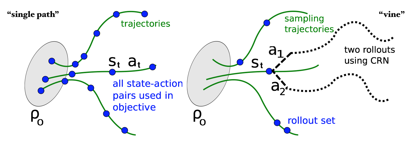
This is exactly the optimization task corresponding to the “single path” sampling scheme in their paper. Another sampling scheme called “vine”, which involves constructing a rollout set and then performing multiple actions from each state in the rollout set. It can reduce variance in estimation, while it requires the environment reset to an arbitrary state and therefore is not suitable for the model-free reinforcement learning.

They solve the constrained optimization problem above by following procedure:

1. Calculate the first-order approximation to the objective \(f(x)\) by expanding in the Taylor series around the current point \(x=\theta\), i.e., \(f(\theta')\approx f(\theta) + g^Ts\), where the \(m\) dimensional vectors \(g = \nabla_{x=\theta}f(x)\) and \(s = \theta'-\theta\).
2. Use Fisher information matrix to calculate the quadratic approximation to the KL divergence constraint as \(\mathtt d_{KL}^{\rho_{\pi_{\theta}}}(\pi_\theta, \pi_{\theta'}) \approx \frac{1}{2}s^TBs\), where \(B_{ij} = \frac{\partial}{\partial \theta_i'}\frac{\partial}{\partial \theta_j'} \mathtt d_{KL}^{\rho_{\pi_{\theta}}}(\pi_\theta, \pi_{\theta'})\).
3. Determine the update direction by approximately solving equation \(Bs=g\) with the conjugate gradient method. This step actually changes the optimization objective as \(f(\theta+s) + \mathtt d_{KL}^{\rho_{\pi_{\theta}}}(\pi_\theta, \pi_{\theta+s}) \approx f(\theta) + g^Ts + \frac{1}{2}s^TBs\), which is quite similar to the optimization objective we obtained from policy improvement bound directly but without a coefficient on KL regularizer.
4. Having computed the search direction \(s\approx B^{-1}g\), we compute the maximal step size \(\beta\) such that \(\theta+\beta s\) satisfies the KL divergence constraint. That is an upper bound on it, \(\Delta \geq \mathtt d_{KL}^{\rho_{\pi_{\theta}}}(\pi_\theta, \pi_{\theta+s}) \approx \frac{1}{2}(\beta s)^T B (\beta s) = \frac{1}{2} \beta^2 s^TBs\). We have \(\beta \leq \sqrt{2\Delta/s^TBs}\).
5. Perform the line search on the objective \(f(\theta + \beta s)+\chi[\mathtt d_{KL}^{\rho_{\pi_{\theta}}}(\pi_\theta, \pi_{\theta+\beta s}) \geq \Delta]\) by shrinking \(\beta\) exponentially until the objective improves, where \(\chi[\dots]\) equals 0 when its assertion is satisfied and \(+\infty\) otherwise.

After performing these five steps, we finish one iteration and obtain a return \(\pi_{\theta'} = \pi_{\theta + \beta s}\) as the new policy which approximately guarantees a non-increasing improvement of the expected cumulative cost.