We propose a novel approach of imitation refinement, which improves the quality of imperfect patterns, by mimicking the characteristics of ideal data. We demonstrate the effectiveness of imitation refinement on two real-world applications: in the first application, we show imitation refinement improves the quality of poorly written digits by imitating typesetting or well-written digits. In the second application, we show that imitation refinement improves the quality of identified crystal patterns from X-ray diffraction data in materials discovery.
Abstract
Many real-world tasks involve identifying patterns from data satisfying background and prior knowledge, for which the ground truth is not available, but ideal data can be obtained, for example, using theoretical simulations. We propose a novel approach, imitation refinement, which refines imperfect patterns by imitating ideal patterns. The imperfect patterns are obtained for example using an unsupervised learner. Imitation refinement imitates ideal data by incorporating prior knowledge captured by a classifier trained on the ideal data: an imitation refiner applies small modifications to imperfect patterns, so that the classifier can identify them. In a sense, imitation refinement fits the data to the classifier, which complements the classical supervised learning task. We show that our imitation refinement approach outperforms existing methods in identifying crystal patterns from X-ray diffraction data in materials discovery. We also show the generality of our approach by illustrating its applicability to a computer vision task.
Socratic Dialogue
Q: I’m curious about imitation refinement. Could you explain it?
Suppose that we have an imperfect dataset \(A\), whose members come from post-processing a real physical experiment or a complete unsupervised learning approach. Members in the imperfect dataset are defective because they fail to satisfy feasible conditions. On the other hand, we have an ideal dataset \(E\), whose members satisfy all physical constraints and prior knowledge. Our goal is to modify the members in the imperfect dataset \(A\) so that they imitate the characteristics of the members in the ideal dataset \(E\).
Formally, consider we trained an ideal classifier \(\mathcal C\) to classify entities in the ideal dataset \(E\), which captures the prior knowledge from an idealized world. The imitation refinement modifies examples from the imperfect dataset \(A\) so the classifier \(\mathcal C\) identifies them. We search for an optimal refiner \(\mathcal R\) to refine samples \(x\)’s drawn from the imperfect dataset \(A\), such that \(\mathcal C\) has better performance on the refined dataset \(\mathcal R(A) = \{R(x) | x\in A\}\).
Q: What do you mean by “better performance”?
We can measure the performance of a classifier \(\mathcal C\) in multiple ways, for example, the confidence of its predictions, or the accuracy if the labels are available. In general, the performance of a classifier \(\mathcal C\) can be measured as its evaluation loss:
\[\eta_{\mathcal C}(A) := \mathbb E_{x\sim A} [\mathcal H(\mathcal C(x))],\]where \(\mathcal H(\cdot)\) is a function giving a low score if the refined samples can be certainly classified in one category in the ideal world. For instance, \(\mathcal H(\cdot)\) can be the cross-entropy when the target categories are given when training, or be the entropy of predictions for some categories, which represents the uncertainty of the ideal classifier \(\mathcal C\) on the refined dataset \(\mathcal R(A)\), in the non-targeted case. We expected a low \(\eta_{\mathcal C}(\mathcal R(A))\) after refinement.
Q: Okay. But why do we want to imitatively refine an imperfect dataset?
For example, in our materials discovery application, the imperfect dataset comprises of candidate patterns that are supposed to correspond to pure crystal structures that are obtained from real XRD data, using unsupervised learning. Each candidate pattern contains information of interest, but often it is mixed with other patterns or corrupted with background noise. On the other hand, we can obtain ideal XRD patterns for known materials from a dataset obtained using simulation. Such patterns are synthesized assuming ideal conditions. We want to imitatively refine the imperfect crystal structure patterns obtained by unsupervised learning to satisfy prior knowledge encapsulated in the ideal dataset.
Q: How is imitation refinement an inverse problem to classification?
One may view the classification and the imitation refinement problems as mappings between a space of datasets \(\mathbb D\) and a model space \(\mathbb M\), see this figure:
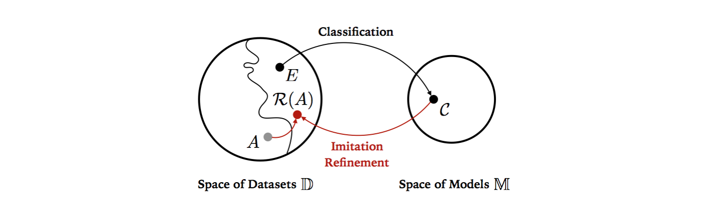
Given a dataset \(E \in \mathbb D\), in classification problem we try to find a classifier \(\mathcal C \in \mathbb M\) such that some efficacy loss \(\eta_{\mathcal C}(E)\) is low. Conversely, In hypothetical refinement problem, given a well trained classifier \(\mathcal C \in \mathbb M\), we are interested in searching for a optimal dataset \(\mathcal R(A)\) in \(\mathbb D\) to make model efficacy loss \(\eta_{\mathcal C}(\mathcal R(A))\) lower, where \(A \in \mathbb D\) is a poor initially given dataset and mapping \(\mathcal R: \mathbb D \rightarrow \mathbb D\) is a refinement.
Q: There seems to be much possible refinement. Which one is “optimal” in your definition?
The “simplest” one. We expect \(\mathcal R\) modify the original data as little as possible to accomplish its goal. The simplicity of refinement can be measured by a discrepancy distance:
\[\delta_{\mathcal C}(A, \mathcal R(A)):= \mathbb E_{x\sim A}[\delta_{\mathcal C}(x, \mathcal R(x))].\]In general, \(\delta_{\mathcal C}\) is a differentiable user-defined metric which measures the degree to which \(\mathcal R\) modifies \(x\). One option is to use a metric on the input space such as \(\ell_p\)-norm. In some cases, a distance metric based on higher level features can be more meaningful, such as features extracted from intermediate layers from a neural network.
Q: Okay. I now understand the optimal imitation refinement is the simplest refinement among all of those making the classifier effective on the refined dataset. But how do you find it?
We can convert it into an optimization problem
\[\begin{eqnarray} \min_{\mathcal R} && \delta_{\mathcal C}(A, \mathcal R(A))\\ \textrm{s.t.} && \mathcal R \in \arg \min_{\mathcal R} \eta_{\mathcal C}(\mathcal R(A)) \end{eqnarray}\]We may relax the condition by minimizing the evaluation loss at the same time to obtain a single optimization problem:
\[\min_{\mathcal R} (1-\lambda) \delta_{\mathcal C}(A, \mathcal R(A))+\lambda\eta_{\mathcal C}(\mathcal R(A)),\]where \(\lambda\) is a weight that trades off the refinement simplicity and the model effectiveness.
Visual Results of Refining Hand-Written Digits

Visual results of imitation refinement: (a) Selected examples of test results of targeted refinement on the imperfect hand-written digits. We set \(\lambda = 0.55\) in the experiment to balance the discrepancy loss and the evaluation loss. In the first row, the target is “6” while the original imperfect digit is not complete. The refiner improves this digit by completing it. In the second row, the target is “7” while the original imperfect digit is like a “2”. The refiner corrects this digit by erasing its redundant part.
A more interesting example of a batch of test results of non-targeted imitation refinement on the poorly written digits is shown in (b). The refiner modifies original ambiguous digits to the ones with higher classifier certainty. We set \(\lambda = 0.15\) for this case. Since the process is non-targeted, it can creatively refine a digit to the less confusing one in the classifier’s sense. Four interesting instances are displayed in the left figure: 1) The first row shows an imperfect digit originally classified as “1”, being refined to a more idealized “7” by enhancing the horizontal line on the top, which corresponds with the human label. 2) The second row shows an imperfect digit correctly labeled originally as “4” but it may also be a “1” or “9”, since its left part is blurred. By erasing its left part, it becomes a more certain “1”. 3) An ambiguous digit which looks like “8”, “3” and “0” is shown in the third row, whose human label is “0”, while the classifier identifies it as “8”. To increase the certainty, its left connected line is erased after refinement, and it is more like a digit “3”. 4) In the last row, an imperfect digit “2” is so much like “7” that the classifier misclassified it. The refiner reinforces the classifier’s opinion by extending the vertical line in the middle and fading the connecting line.
Authors
Runzhe Yang*, Junwen Bai* (equal authorship), Yexiang Xue and Carla Gomes.