How Does Value-Based Reinforcement Learning Find the Optimal Policy?

DeepMind researchers claimed state-of-the-art results in the Arcade Learning Environment in their recent ICML paper “A Distributional Perspective on Reinforcement Learning”. They investigate a distributional perspective of the value function in the reinforcement learning context and further design an algorithm applying Bellman’s equation to approximately learn value distributions, which results in better policy optimization. The discussion in their paper follows closely the classical analysis of Bellman operator and dynamic programming, which should be familiar to most AI researchers.

In this article, I will introduce the mathematical background of the classical analysis of reinforcement learning, that is, the Bellman operator is essentially a contraction mapping on a complete metric space, and explain how value-based reinforcement learning, e.g. Q-learning, finds the optimal policy. Based on these general ideas, readers will see how straightforward the idea that the DeepMind paper comes up with, and hopefully draw some inspiration from this topological perspective to design future RL algorithms.

For the reader who prefers to systematically learn from books, I strongly recommend you to read the textbook Linear Operator Theory in Engineering and Science for acquiring mathematical background, and the book Abstract Dynamic Programming by Dimitri P. Bertsekas to study the connection between contraction mapping and dynamic programming. If you don’t remember Markov decision processes or policy optimization in reinforcement learning, my previous blog has introduced them briefly.

• Topology of Metric Spaces
  • Cauchy Sequences and Completeness
  • Contraction Mapping Theorem
• Contractive Dynamic Programming
  • Contraction Property
  • Monotonicity Property
• Value-Based Reinforcement Learning
  • Approximate Value Iteration
  • Approximate Policy Iteration
  • Q-Learning: Asynchronous Value Iteration
• A Methodology for Developing Iterative RL Algorithms
  • Learning from Value Distribution
  • Multi-Objective RL
• Summary: Contraction, Value Iteration, and More

Topology of Metric Spaces

Literally, the word “topology” means “the study of spatial properties”. The space here could be any abstract space with certain properties. A natural way for us to quickly start the discussion is to observe a metric space.

Definition 1. (Metric Space) A metric space is an ordered pair \((X, d)\) consists of an underlying set \(X\) and a real-valued function \(d(x, y)\), called metric, defined for \(x, y \in X\) such that for any \(x, y, z \in X\) the following conditions are satisfied:

1. \(d(x, y) \geq 0\)                          [non-negativity]
2. \(d(x, y) = 0 \Leftrightarrow x = y\)         [identity of indiscernibles]
3. \(d(x, y) = d(y, x)\)                 [symmetry]
4. \(d(x, y) \leq d(x, z) + d(z, y)\) [triangle inequality]

All these four conditions are in harmony with our intuition of distance. Indeed, the Euclidean distance \(d(x, y) = \sqrt{(x_1 - y_1)^2 + (x_2 - y_2)^2 + (x_3 - y_3)^2}\) is a valid metric.

Cauchy Sequences and Completeness

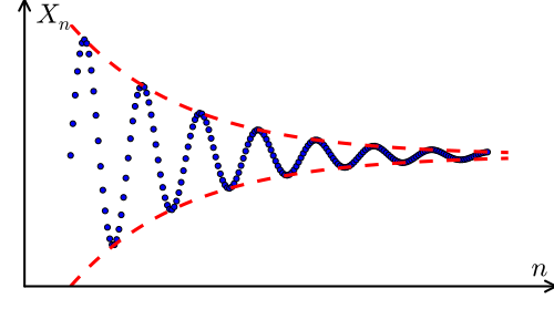
When we construct a metric space \((X, d)\), it is common to expect our metric space has no “point missing” from it. For example, the space \(\mathbb Q\) of rational numbers, with the metric by the absolute value \(|\cdot|\) of the difference, is not complete. Just consider the rational sequence \(x_{n+1} = \frac{x_n}{2} + \frac{1}{x_n}\), \(x_1 = 1\), whose elements become arbitrarily close to each other as the sequence progresses, but it doesn’t converge to any point in space \(\mathbb Q\). Therefore, the space \(\mathbb Q\) is incomplete, since it obviously misses points.

A sequence like that in our example is called Cauchy sequence. Formally, we define the Cauchy sequence in and the completeness of a metric space \((X, d)\) as follows:

Definition 2. (Cauchy Sequence) A sequence \(\{x_n\}\) is said to be Cauchy sequence if for each \(\epsilon > 0\) there exists an \(N_\epsilon\) such that \(d(x_n, x_m) \leq \epsilon\) for any \(n, m \geq N_\epsilon\).

Definition 3. (Complete Metric Space) A metric space is said to be complete if each Cauchy sequence is a convergent sequence in it.

The significance of complete metric space is difficult to be overemphasized. In many application, it is easier to show a given sequence is a Cauchy sequence than to show it is convergent. However, if the underlying metric space is complete, to show a given sequence is a Cauchy sequence is sufficient for convergence.

Contraction Mapping Theorem

Now we introduce the contraction mapping based on the concept of completeness.

Definition 4. (Contraction) Let (X, d) be a metric space and \(f: X \rightarrow X\). We say that \(f\) is a contraction, or a contraction mapping, if there is a real number \(k \in [0, 1)\), such that \[ d(f(x), f(y)) \leq kd(x,y) \] for all x and y in X, where the term \(k\) is called a Lipschitz coefficent for \(f\).

The reason that contractions play an important role in dynamic programming problems lies in the following Banach fixed-point theorem.

Theorem 1. (Contraction Mapping Theorem) Let \((X, d)\) be a complete metric space and let \(f: X \rightarrow X\) be a contraction. Then there is one and only one fixed point \(x^*\) such that \[ f(x^* ) = x^* . \] Moreover, if \(x\) is any point in \(X\) and \(f^n(x)\) is inductively defined by \(f^2(x) = f(f(x))\), \(f^3(x) = f(f^2(x)), \dots, f^n(x) = f(f^{n-1}(x))\), then \(f^n(x) \rightarrow x^*\) as \(n \rightarrow \infty\).

proof. Let us first prove every sequence \(\{f^n(x)\}\) convergent to a fixed point. Since the metric space \((X, d)\) is complete, we only need to prove every \(\{f^n(x)\}\) is a Cauchy sequence. By the triangle inequality and symmetry of metric, for all \(x, y \in X\),

Consider two points \(f^\ell(x)\), \(f^m(x)\) in the sequence. Their distance is bounded by

since \(k \in [0, 1)\) the distance converges to zero as \(\ell, m \rightarrow \infty\), proving that \(\{f^n(x)\}\) is a Cauchy sequence. Because the space \((X, d)\) is complete, \(\{f^n(x)\}\) converges.

We now show that \(x^* = \lim_{m\rightarrow \infty} f^m(x)\) is a fixed point, and it is unique. Since \(f\) is a contration, by definition it is continous. Therefore \[ f(x^* ) = f(\lim_{m\rightarrow \infty} f^m(x)) = \lim_{m\rightarrow \infty} f(f^m(x)) = \lim_{m\rightarrow \infty} f^m(x) = x^* . \] The uniqueness of \(x^*\) can be proved by contradiction. Assume \(x^*\) and \(y^*\) are two distinct fixed points of \(f\). We then get the contradiction \[ 0 < d(x^* , y^* ) = d(f(x^* ) , f(y^* )) \leq k d(x^* , y^* ) < d(x^* , y^* ). \] Hence \(f\) has only one fixed point and \(\{f^n(x)\}\) converges to it for any \(x \in X\). \(\blacksquare\)

Contractive Dynamic Programming

The contractive dynamic programming model is introduced by Eric V. Denardo in 1967, which applies contraction theorem to a broad class of optimization problems. It captures two widely shared properties of the optimization problem, contraction and monotonicity properties to develop a high level abstraction of optimization methods.

Some terminology is now introduced. Let \(S\), \(A\) be two sets, which we refer to as a set of “states” and a set of “actions”, respectively. For each \(s \in S\), let \(A_s \subseteq A\) be the nonempty subset of actions that are feasible at state \(s\). We denote by \(\Pi\) the set of all stationary deterministic policies \(\pi: S \rightarrow A\), with \(\pi(s) \in A_s\), for all \(s \in S\).

To introduce return function, let \(V\) be the set of all bouned real valued functions from \(S\) to reals, and let \(H: S\times A \times V \rightarrow \mathbb R\) be a given mapping. One might think \(H(s, a, v)\) as the total payoff for starting at state \(s\) and choosing action \(a\) with the prospect of receiving \(v(s')\) if the transition \((s, a)\rightarrow s'\) is happened. We consider the operator \(\mathcal T_\pi: V \rightarrow V\) defined by \[ (\mathcal T_\pi v)(s) := H(s, \pi(s), v), ~\forall s\in S, v\in V, \] and we also consier the operator \(\mathcal T\) defined by \[ (\mathcal T v)(s) := \sup_{a \in A_s}H(s, a, v), ~\forall s\in S, v\in V. \] We call \(\mathcal T_\pi\) the “evaluation operator” and \(\mathcal T\) the “optimality operator”. Our goal is to find a policy maximizing our total payoff. Following two properties provide conditions under which our goal can be realized by iteratively applying these two operators.

Contraction Property

Let a metric \(d\) on \(V\) is defined by \(d(u, v) = \sup_{s \in S} |u(s) - v(s)|\). Using the fact \(V\) is a space of bounded functions, it is easy to show that the metric space \((V, d)\) is complete.

Assumption 1. (Contraction) For all \(u, v \in V\) and \(\pi \in \Pi\), for some \(\gamma \in [0, 1)\), we have \[ d(\mathcal T_{\pi} u, \mathcal T_{\pi} v) \leq \gamma d(u ,v). \]

Proposition 1. Suppose the contraction assumption is satisfied. Then \(\mathcal T\) is also a contraction with the same Lipschitz coefficient \(\gamma\).

Proof. Consider arbitrary \(u, v\) and we can write \((\mathcal T_\pi u) (s) \leq (\mathcal T_\pi v)(s) + \gamma d(u, v)\) for each \(\pi \in \Pi\) by assumption. For any fixed state \(s\), we take supremum of both side over \(\pi \in \Pi\), we have \[ \sup_{\pi\in\Pi} \left\{(\mathcal T_\pi u) (s)\right\} = \sup_{\pi(s) \in A_s}H(s, \pi(s), v) = (\mathcal T u) (s) \leq (\mathcal T v)(s) + \gamma d(u, v) \] Reversing the rolee of \(u\) and \(v\), we have \((\mathcal T v) (s) \leq (\mathcal T u)(s) + \gamma d(u, v)\) for any fixed state \(s\). Jointly, we have proved \(|(\mathcal T u)(s) - (\mathcal T v) (s)| \leq \gamma d(u, v)\) for all \(s\in S\). Hence, \[ d(\mathcal T u, \mathcal T v) = \sup_{s\in S} |(\mathcal T u)(s), (\mathcal T v)(s)| \leq \gamma d(u, v). \] The optimality operator \(\mathcal T\) is also a contraction with Lipschitz coefficient \(\gamma\). \(\blacksquare\)

The Banach fixed-point theorem guarantees that iteratively applying evaluation operator \(\mathcal T_\pi\) to any function \(v \in V\) will converge to a unique function \(v_\pi\) in \(V\) such that \[ v_\pi(s) = H(s, \pi(s), v_\pi), ~~ \text{for each}~ s \in S. \] The function \(v_\pi\) is called value fuction of the policy \(\pi\). The optimal value function \(v_{\mathtt{opt}}\) is defined by \(v_{\mathtt{opt}}(s) := \sup_{\pi\in \Pi} v_{\pi}(s)\) for all \(s\in S\). Similarly, iteratively applying optimality operator \(\mathcal T\) to any funciton \(v \in V\) will converge to a unique function \(v^* \in V\) such that \[ v^* (s) = \sup_{a\in A_s}H(s, \pi(s), v^* ), ~~\text{for each}~ s \in S. \] How should we interpretate this fixed point \(v^*\)? When does \(v^*\) equal \(v_{\mathtt{opt}}\) that we desire? One may have a sense that \(v_{\mathtt{opt}} \geq v^*\) since the following result aways holds.

Lemma 1. (\(v_{\mathtt{opt}} \geq v^*\)) For any \(\epsilon > 0\), there exists a policy \(\pi_\epsilon\) such that for any \(s\), \(H(s, \pi_\epsilon(s), v^* ) \geq \sup_{a\in A_s} H(s, a, v^* ) - \epsilon (1-\gamma)\), and any such \(\pi_\epsilon\) satisfies \(v_{\pi_\epsilon} \geq v^* - \epsilon\).

Proof. Note that for any \(v \in V\) and \(\pi\in\Pi\), we have an upper bound

Now let \(v = v^*\), and \(\pi = \pi_{\epsilon}\) such that \(H(s, \pi_\epsilon(s), v^* ) \geq \sup_{a\in A_s} H(s, a, v^* ) - \epsilon (1-\gamma)\) for any \(s\), we have \(d(v_{\pi_{\epsilon}}, v^* ) \leq \epsilon\). \(\blacksquare\)

If we can show the reverse inequality, \(v^* \geq v_{\mathtt{opt}}\) , then we conclude \(v^* = v_{\mathtt{opt}}\). However, it does not always hold true. A sufficient condition, monotonicity property, is therefore introduced to make them identical.

Monotonicity Property

Assumption 2. (Monotonicity) For \(u, v \in V\), if \(u \geq v\), then \(\mathcal T_\pi u \geq \mathcal T_\pi v\) for each \(\pi\in \Pi\), where we write \(u \geq v\) if \(u(s) \geq v(s)\) for each state \(s\), and \(u > v\) if \(u \geq v\) and \(u \neq v\).

The monotonicity property was introduced by L. G. Mitten in 1964. There are many value functions, including the one in the infinite horizon MDP, have the monotonicity property. The following theorem shows why the contraction and monotonicity properties are important in the contractive dynamic programming model.

Theorem 2. Suppose the contraction and monotonicity properties hold. Then \(v^* = v_{\mathtt{opt}}\).

Proof. Note that \(H(s, \pi(s), v^* ) \leq \sup_{a \in A_s} H(s, a, v^* )\) for any \(s\in S\) and \(\pi \in \Pi\). It means \(\mathcal T_{\pi} v^* \leq \mathcal T v^*\) for all \(\pi\). Repeatedly applying the monotonicity property \(k\) times, we derive \(\mathcal T_{\pi}^k v^* \leq \cdots \leq \mathcal T_{\pi}^2 v^* \leq \mathcal T_{\pi} v^* \leq \mathcal T v^* = v^*\). By contraction property \(\lim_{k\rightarrow \infty}\mathcal T_{\pi}^k v^* = v_{\pi}\). Therefore \(v_{\pi} \leq v^*\) for any \(\pi\) and \(v_{\mathtt{opt}} \leq v^*\). On the other hand, by Lemma 1 which utilizes the contraction property we have \(v^* - \epsilon \leq v_{\pi_{\epsilon}} \leq v_{\mathtt{opt}}\) for any \(\epsilon > 0\). Jointly, \[ v^* - \epsilon \leq v_{\mathtt{opt}} \leq v^* \] for any \(\epsilon > 0\). This implies \(v^* = v_{\mathtt{opt}}\) and completes the proof. \(\blacksquare\)

Value-Based Reinforcement Learning

Reinforcement learning (RL) approximates the optimal policy of a Markov decision process. This method succeeded in solving many challenging problems in diverse fields, such as robostics, transportation, medicine, and finance. Many RL methods are considered by the classic textbook Reinforcement Learning: An Introduction by Richard S. Sutton and Andrew G. Barto (We are translating its latest version into Chinese!).

Roughly speaking, the value (function) based reinforcement learning is a large category of RL methods which take advantage of the Bellman equation and approximate the value function to find the optimal policy, such as SARSA and Q-Learning. By contrast, the policy-based reinforcement learning methods directly optimize the quantity of total reward, e.g. REINFORCE, which are more stable but less sample efficient than value-based methods.

The key idea of value-based RL relates two Bellman equations of an infinite horizon discounted MDP \(\mathcal M = \langle S, A, \mathcal R, \mathcal P, \gamma \rangle\), where \(\mathcal R(s, a)\) is the immediate reward function, and \(\mathcal P(s'|s, a)\) is the probabilistic transition model, and \(\gamma\) is the discount factor (If you just forget the definition of MDPs, please refer to my previous blog). The first equation is so-called Bellman expectation equation: \[ v_{\pi}(s) = R(s, \pi(s)) + \gamma \sum_{s’ \in S} \mathcal P(s’ | s, \pi(s))\cdot v_{\pi}(s’). \] This equation describe the expected total reward for taking the action prescribed by policy \(\pi\). The other equation is called Bellman optimality equation: \[ v^* (s) = \max_{a\in A} \left\{R(s, a) + \gamma \sum_{s’ \in S} \mathcal P(s’ | s, a)\cdot v^* (s’)\right\}. \]

Now we consider two corresponding operators, defined by the following \[ (\mathcal T_{\pi}v)(s) := R(s, \pi(s)) + \gamma \sum_{s’ \in S} \mathcal P(s’ | s, \pi(s))\cdot v(s’) ~~~\text{[Bellman evaluation operator]}, \] and \[ (\mathcal Tv)(s) := \max_{a\in A} \left\{ R(s, a) + \gamma \sum_{s’ \in S} \mathcal P(s’ | s, a)\cdot v(s’) \right\} \text{[Bellman optimality operator]} \] for any value function \(v \in V\). Note that \(v_{\pi}\) and \(v^*\) are fixed points of operator \(\mathcal T_{\pi}\) and \(\mathcal T\) respectively. If we can show that \(\mathcal T_{\pi}\) satisfies both contraction and monotonicity properties, according to results we have drawn in the last section, \(v^\pi\) and \(v^*\) are unique fixed points that repeatedly applying \(\mathcal T_{\pi}\) and \(\mathcal T\) will converge to respectively, and \(v^* = v_{\mathtt{opt}}\).

Proposition 2. The contraction and monotonicity properties hold for Bellman evaluation operator \(\mathcal T_{\pi}\) for any stationary policy \(\pi \in \Pi\).

Proof. For any value functions \(u, v \in V\), and any policy \(\pi \in \Pi\), we have

Therefore \(\mathcal T_{\pi}\) is a contraction with Lipschitz coefficient \(\gamma\). The contraction property holds. According to Proposition 1, the optimality operator \(\mathcal T\) is also an \(\gamma\)-contraction.

Further more, for any value functions \(u \geq v\), we have \[ (\mathcal T_{\pi} u)(s) - (\mathcal T_{\pi} v)(s) = \gamma \sum_{s’ \in S} \mathcal P(s’ | s, \pi(s))\cdot (u(s’) - v(s’)) \geq 0 \] for all \(s \in S\). Hence \(\mathcal T u \geq \mathcal T v\). The monotonicity property holds. \(\blacksquare\)

Approximate Value Iteration

As the discussion above indicates, if the model is known, one can design an policy optimization algorithm by generating \(\mathcal T v, \mathcal T^2 v, \dots\) which converges to \(v^*\) and then extracting the corresponding optimal policy. This is exactly the value iteration (VI) method. This algorithm simply starts with any value function guess and repeatedly apply the Bellman optimality operator on it to obtain the optimal value function. Sometimes VI method may be implementable only by approximation, e.g., when the state space \(S\) is extremely large or when the value function is updated by some constant step size. A common solution is depicted as the following approximate value iteration algorithm.

# Approximate Value Iteration 
Initialize value function v arbitrarily.
Repeat:
    Update v, such that sup|v-T(v)| ≤ δ
until v converges
Extract a policy: π, such that sup|T_π(v) - T(v)| ≤ ϵ

By applying the triangle inequality and the contraction property of \(\mathcal T_{\pi}\) and \(\mathcal T\), we can assert the error bounds for the output value function \(v_{\mathtt{final}}\), which is bounded by \(d(v_{\mathtt{final}}, v_{\mathtt{opt}} ) \leq \frac{\delta}{1 - \gamma}\), and the extracted policy \(\pi_{\mathtt{final}}\), whose value is bounded by \(d(v_{\pi_{\mathtt{final}}}, v_{\mathtt{opt}} ) \leq \frac{\epsilon}{1 - \gamma} + \frac{2\gamma\delta}{(1-\gamma)^2}\) (proof is straightforward, check them yourself :-)). The VI algorithm converges exponentially when \(\epsilon = 0\) and \(\delta = 0\).

Approximate Policy Iteration

The VI method is a direct creation based on the fact that the Bellman optimality operator \(\mathcal T\) is a contraction. However, people may think by involving policy evaluation each step one can have a better rate of convergence and a better approximation of optimal policy, though it will incur more calculation each iteration. This is plausible, but not insignificantly so in theory. The approximate policy iteration (PI) algorithm is stated as follows:

# Approximate Policy Iteration
Given the current policy π_k
Repeat:
    Policy evaluation: Compute v such that
        sup|v - (T_π_k)^m_k (v) | ≤ δ
    by appying Bellman evaluation operator T_π

    Policy improvement: Extract a policy π_{k+1} that satisfies
        sup|T_π_{k+1}(v)- T(v)| ≤ ϵ
    π_k ← π_{k+1}
until v converges.
Extract π_{k+1} 

In this algorithm, the parameter \(m_k\) is an positive intergers. Taken the usual choice of \(m_k = 1\), we can show that \(d(v_{\pi_{k+1}}, v_{\mathtt{opt}}) \leq \gamma d(v_{\pi_{k}}, v_{\mathtt{opt}}) + \frac{\epsilon + 2\delta\gamma}{1 - \gamma}\) for each iteration. Therefore, its final error bound is asymptotically proportional to \(1/(1-\gamma)^2\), which indicates PI does not hold an accuracy advantage over VI. And the exact PI converges at an exponential rate which is as same as that of exact VI.

Q-Learning: Asynchronous Value Iteration

In the last two section we explained how we do classical model based planing for MDPs from the topological point of view. Many readers by now have a sense that how this stuff and value-based reinforcement learning are connected. But there remains a critical question: Can this explanation is still suitable for those general model free cases? Can we explain those classical reinforcement “learning” algorithm, such as Q-learning, in an analog way?

Intuitively, the answer should be “yes”. Consider the evaluation operator \(\mathcal T_{\pi}\) and optimality operator \(\mathcal T\) defined by \[ (\mathcal T_{\pi} q)(s, a) := R(s, a) + \gamma\mathbb E_{\mathcal P, \pi} q(s’, a’) \] and \[ (\mathcal T q)(s, a) := R(s, a) + \gamma\mathbb E_{\mathcal P} \max_{a’\in A} q(s’, a’) \] respectively, over the Q value function space \(\mathbb R^{S\times A}\), with the similar metric as that of \(V\). Following the similar analysis, the contraction and the monotonicity properties hold for them. However, since the model is unknown, we cannot update the Q value function as that in value iteration. We can only approximate and update the Q value for some certain pair \((s, a)\) by sampling or temporal difference method each iteration. Is its convergence still guaranteed? The following theorem resolves our doubts.

Definition 5. (Asynchronous Value Iteration) Conside value function \(v\) as a composition of \((v_s)_ {s\in S}\) such that in each iteration, \[ v_s^{t+1}(s’) = \begin{cases} \mathcal Tv^{t}(s’), & \text{if}~s’ = s\newline \mathcal v_s^{t}(s’), & \text{otherwise.} \end{cases} \] Theorem 3. (Asynchronous Convergence Theorem) If each restricted value function \(v_s\) can be update infinite times, and there is a sequence of nonempty subsets \(\{V^k\} \subseteq V\) with \(V^{k+1}\subseteq V^{k}\), \(k = 0, 1, \dots\) such that if \(\{v^k\}\) is any sequence with \(v_k\in V_k\) for all \(k \leq 0\), the \(\{v^k\}\) converges pointwise to \(v^*\). Assume further the following:

1. Synchronous Convergence Condition: We have \[ \mathcal T v \in V^{k+1}, \forall v \in V^k \]
2. Box Condition: For all \(k, V^k\) is a Cartesian product of the form \[ V^k = \times_{s\in S} V_s^k \]

where \(V_{s}^k\) is a set of bounded real-valued functions on state \(s\). Then for every \(v^0 \in V^0\) the sequence \(\{v^t\}\) generated by the asynchronous VI algorithm converges to \(v^*\).

Proof. To show that the algorithm converges is equivalent to show that the iterates from \(V^k\) will get in to \(V^{k+1}\) eventually, i.e., for each \(k \leq 0\), there is a time \(t_k\) such that \(v^t\in V^{k}\) for all \(t \geq t_k\). We can prove it by mathematical induction.

When \(k = 0\), the statement is true since \(v^0\in V^0\). Assuming the statement is true for a given \(k\), we will show there is a time \(t_{k+1}\) with the required properties. For each \(s\in S\), let set \(L_{s} = \{t: s^t = s\}\) record the time an update happend on the state \(s\). Let \(t(s)\) be the first element in \(L_{s}\) such that \(t(s) \geq t_{k}\). Then by the synchrnous convergence condition, we have \(\mathcal Tv^{t(s)} \in V^{k+1}\) for all \(s\in S\). In the view of the box condition, it implies \(v^{t+1}(s)\in V_s^{k+1}\) for all \(t \geq t(s)\) for any \(s\in S\). Therefore, let \(t_{k+1} = \max_{s}t(s) + 1\), using the box condition, we have \(v^t \in V^{k+1}\) for all \(t \leq t_{k+1}\). By mathematical induction, the statement holds, and \(V^k\) will get in to \(V^{k+1}\) eventually. Hence, \(\{v^t\}\) converges to \(v^*\). \(\blacksquare\)

A Methodology for Developing Iterative RL Algorithms

It is really exciting to see that the convergence and correctness of value-based reinforcement learning algorithm, such as Q-learning, can be interpreted in a topological view. In fact, the contraction mapping theory provides us with a methodology for developing iterative value-based RL algorithm. In a high-level overview, iterative value-based RL algorithms are concerned with the following five essential elements:

• Value Space \(V\): A common choice of \(V\) is the space of value functions in \(\mathbb R^S\) or the space of Q-value functions in \(\mathbb R^{S\times A}\). There are many other choices such as the space of ordered pair of \((V,Q)\) (Example 2.6.2 in Dimitri’s book), or the space of multi-dimensional value functions.

• Value Metric \(d\): It defines the “distance” between two points in the value space. Besides the basic four conditions, the metric \(d\) should ensure a complete metric space \((V, d)\) to validate the Banach’s fixed-point theorem. A compatible selection of value metric will make our analysis much easier.

• Evaluation Operator \(\mathcal T_{\pi}\): We have constructed a recursive expression of a certain value point in the value space associated with some policy, e.g., the Bellman expectation equation, \[ v_{\pi}(\cdot) = H(\cdot, \pi(\cdot), v_{\pi}) \] to depict the value of a policy \(v_{\pi}\) as a fixed point we desire. Carefully verify that the contraction and the monotonicity properties hold for \(\mathcal T_{\pi} v:=H(\cdot, \pi(\cdot), v)\).

• Optimality Operator \(\mathcal T\): Write down recursive expression of the optimal point in the value space, e.g., the Bellman optimality equation, \[ v^* (\cdot) = \sup_{\pi\in \Pi}\mathcal T_{\pi} v^* (\cdot). \] One thing important is to make sure the contraction property holds for the optimality operator \(\mathcal T:= \sup_{\pi\in \Pi}\mathcal T_{\pi}v\). Note that when the metric \(d\) is the supremum of the absolute value of the difference, the contraction property of \(\mathcal T\) is automatically satisfied according to Proposition 1.

• Updating Scheme: It is the most tricky part. For those small-scale problems, the asynchronous value iteration is enough. However, to make our reinforcement learning algorithm practical and scalable, we have to consider much more factors. For example: Should our algorithm be on-policy or off-policy? How do we approximate the value and policies? If it is an online algorithm, how do we trade off exploration and exploitation? All these details will significantly influence the performance of our algorithm on real-world tasks.

Learning from Value Distribution

Let’s get back to the DeepMind paper mentioned at the begining, which proposes a new reinforcement learning algorithm from a distributional perspective. This work is actually a good example of developing and analyzing a new reinforcement learning algorithm using the methodology that we summarize above.

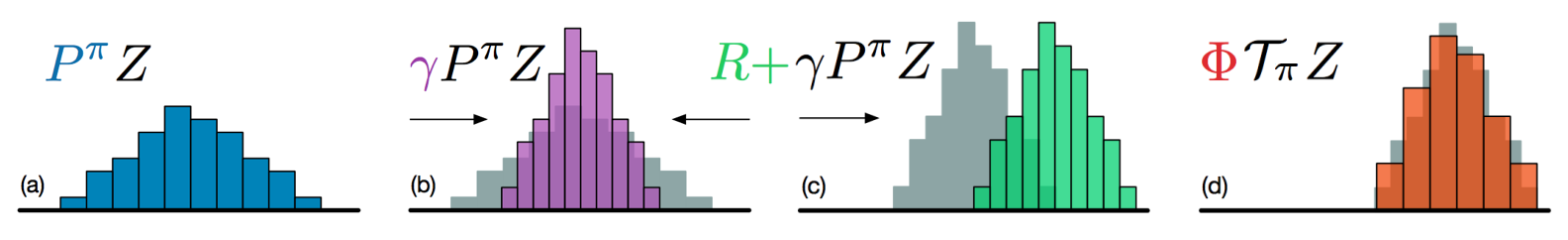
In this example, the value space consists of all the “value distribution” \(Z(s, a)\). The value metric of the value space is defined by \(d(Z_1, Z_2):= \sup_{s, a}d_{w}(Z_1(s,a), Z_2(s,a))\), where \(d_{w}\) is the Wasserstein distance between two random variables. The evaluation operator is defined by \[ \mathcal T_{\pi} Z(s, a) \stackrel{D}{:=} R(s, a) + \gamma P^{\pi}Z(s, a), \] which is proved to be a contraction in \((\mathcal Z, d)\), where “\(\stackrel{D}{=}\)” means random variables on both sides are drawn from the same distribution. The monotonicity property also holds as they define the order as the order of the magnitude of expectation (\(Z_1 \leq Z_2 \Leftrightarrow \mathbb E Z_1 \leq \mathbb E Z_2\)). The optimality operator is defined by \(\mathcal T Z := \sup_{\pi}\mathcal T_{\pi}Z\). However, since the relative order is incompatible with the metric, this optimality operator is NOT a contraction in \((\mathcal Z, d)\). They use approximate asynchronous value iteration as the updating scheme, where the value distribution function is approximated by a neural network which outputs a discrete distribution between \([V_\text{MAX}, V_\text{MIN}]\).

If we only consider the space of the first-order moment of the value distribution and the metric \(d_{\mathbb E}(\mathbb E Z_1, \mathbb E Z_2):= \sup_{s, a} |\mathbb E Z_1(s,a) - \mathbb E Z_2(s,a)|\), both \(\mathbb E\mathcal T_{\pi}\) and \(\mathbb E\mathcal T\) are contractions. And this explains why the C51 algorithm works well. However, as for predicting value distribution, I doubt the correctness of directly using the result of value iteration. In my opinion, a policy iteration algorithm would be a better choice here for maintaining value distributions, or we should correct the value distribution function by repeatedly applying evaluation operator after the optimal policy is found.

Multi-Objective RL

Another example which might be helpful for us to understand this methodology is the multi-objective reinforcement learning. And this is also an interesting topic I am recently working on. The value space of this problem should be some multi-dimensional value function. The metric can be extended from that of a normed vector space. If we only want to find one policy resulting a Pareto optimal return, or simply want to find the best policy maximizing the return associated with specific weights, the evaluation operator and the optimality operator are very similar to \(R + \gamma P^{\pi}V\) and \(\sup_{\pi} \{R + \gamma P^{\pi}V\}\) (the \(\sup\{\cdot\}\) is defined by Pareto domination and the order of magnitude of weighted sum, respectively). Designing an updating scheme according to the real problem, we are guaranteed to have a viable algorithm. If we want to find all the policies resulting in a Pareto optimal return, or make the policies controllable, how to represent a collection of policies and write down the corresponding evaluation/optimality operator are very challenging.

Summary: Contraction, Value Iteration, and More

In this article, some topological backgrounds of metric spaces and the Banach fixed-point theorem are first introduced. Based on these mathematical foundations, we investigate the contractive dynamic programming, where the contraction property and the monotonicity property together guarantee a unique optimal solution can be achieved exponentially fast. Bring these ideas to the reinforcement learning context, we can explain and analyze value iteration, policy iteration and Q-learning algorithms in a unified framework. It further inspires us to develope a methodology for developing iterative value-based reinforcement algorithm, which requires us to consider value space, value metric, evaluation operator, optimality operator and updating scheme.

The next time someone asks, “how does a value-based RL algorithm converge?”, or “how do people come up with a new RL algorithm?”, we can answer him not first by complex, detailed mathematical deduction, but simply by drawing an intuitive picture and analyzing on those accessible abstractions! Our journey on the topic of topological explanation of value-based reinforcement learning comes to an end here. Hope you enjoyed it!