Neural Dynamics of an E-I Network

We investigate the neural dynamics in an exicitatory-inhibitory neural nerwork (E-I network) with ReLU activation and Hebbian learning. By local bifurcation analysis, we find there are ten possible neural dynamical patterns between one excitatory neuron and one inhibitory neuron with all four types of synaptic connections. The unstable node never exists in this system, and when there is no external input, Hebbian learning makes the network dynamic converge to a stable star. We give sufficient and necessary conditions for the exisitence of limit cycles in an E-I network.

E-I Networks

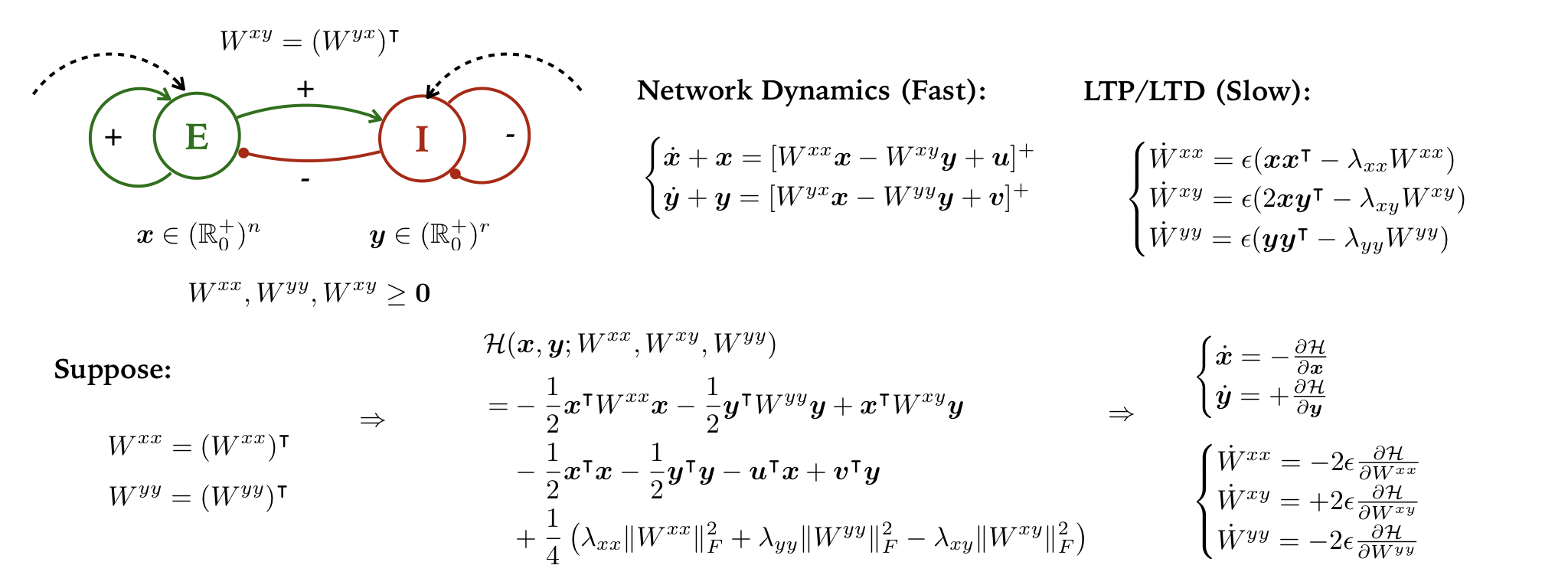
An E-I nerwork consists of two populations of neurons: the excitatory neurons (E) and the inhibitory neurons (I). The E-neurons encourage the firing of the post-synaptic neurons, while the I-neurons resist the firing of the post-synaptic neurons. There are four types of synaptic connections: E-E, E-I, I-E, I-I, with different synaptic weights. We constrain all E-E and I-I connections to be symmetric, and E-I and I-E connections to be anti-symmetric. The weights and neural activity are non-negative. The change of weights is subject to Hebb’s rule. See the general formuation in the above illustration.

Summary

• There are ten possible dynamical patterns for the neural activity of linear neural network by investigating the local bifurcation.
  • All the possible spirals and circles are anticlockwise.
  • The unstable node never exist.
• If there is no external input, in the long term, the fixed point of linear network becomes a stable star.
• The positive fixed point of a linear neural network is also a positive fixed point of its corresponding rectified linear neural network, vise versa.
• There are ten possible dynamical patterns for the neural activity of rectified linear neural network:
  • \(\Delta \neq 0, W^{xx}+W^{yy} < 2W^{xy}\):
    • a. if \(\tau > 0\), i.e., \(W^{xx} > W^{yy}+2\), the fixed point is still an unstable spiral, but there exist one stable limit cycle.
      
    • b. if \(\tau = 0\), i.e., \(W^{xx}=W^{yy}+2\), the fixed point is still a center of circles, but there exist one stable limit cycle.
      
    • c. if \(\tau < 0\), i.e., \(W^{xx} < W^{yy}+2\), the fixed point is still a stable spiral.
  • \(\Delta \neq 0, W^{xx}+W^{yy} = 2W^{xy}\):
    
    • a. if \(\tau > 0\), i.e., \(W^{xx} > W^{yy}+2\), the fixed point is an unstable star.
      
    • b. if \(\tau < 0\), i.e., \(W^{xx} < W^{yy}+2\), the fixed point is a stable star.
  • \(\Delta \neq 0, W^{xx}+W^{yy} > 2W^{xy}\):
    
    • a. if \(\Delta < 0\), i.e., \((W^{xx}-1)(W^{yy}+1) > (W^{xy})^2\),the original fixed point is a saddle point, but there is one boundary stable node.
      
    • b. if \(\Delta > 0\), i.e., \((W^{xx}-1)(W^{yy}+1) < (W^{xy})^2\), we can show that \(\tau < 0\), then the fixed point is a stable node.
  • \(\Delta = 0\): There is no isolated fixed points.
    
    • a. if \(\tau > 0\), i.e., \(W^{xx} > W^{yy}+2\), there is a line repeller.
      
    • b. if \(\tau < 0\), i.e., \(W^{xx} < W^{yy}+2\), there is a line attractor, and one stable node on the boundary.
      
    • c. if \(\tau = 0\), i.e., \(W^{xx}=W^{yy}+2\), there is no fixed points.
• In a rectified linear neural network, if we add two time constants \(\tau_x > 0\) and \(\tau_y > 0\), a limit cycle exists if and only if all the following conditions hold:
    (1) a positive fixed point exists;
    (2) \({\bf \sqrt{\tau_y/\tau_x}\left(W^{xx}-1\right)+\sqrt{\tau_x/\tau_y}\left(W^{yy}+1\right) < 2W^{xy}}\); and
    (3) \({\bf (W^{xx}-1)/\tau_x\geq (W^{yy}+1)/\tau_y}\).
  The behavior of the system when varying \(\tau\) is similar to supercritical Hopf bifurcation.
• When the inhibition is much faster than the excitation, i.e., \(\tau_y/\tau_x \rightarrow 0\), it is impossible to produce limit cycles in an E-I network.

Analysis

CASE 1. the simplest case \(n=r=1\), w/o nonnegative connenction constraints in network dynamics.

Fast Movement (Neural Activity)

The dynamics can be expressed as

where \(W^{xx}, W^{xy}, W^{yy} > 0\), \(x, y, u, v \geq 0\), and \(W^{xy} = W^{yx}\). Then the trace of Jacobian \(\tau = W^{xx}-W^{yy}-2\), the determinant of Jacobian \(\Delta = (W^{xy})^2-(W^{xx}-1)(W^{yy}+1)\). Assume \(\Delta\neq 0\). Using Cramer’s rule, we can rewrite this linear dynamic system as

The external input \(u,v\) control the position of fixed point

The discriminant of this linear system is \(\tau^2 - 4\Delta = (W^{xx}+W^{yy})^2-4(W^{xy})^2\).

Thus, when

• \(\Delta \neq 0, W^{xx}+W^{yy} < 2W^{xy}\):
  
  • a. if \(\tau > 0\), i.e., \(W^{xx}>W^{yy}+2\), the fixed point is an unstable spiral.
    
  • b. if \(\tau = 0\), i.e., \(W^{xx}=W^{yy}+2\), the fixed point is a center of circles.
    
  • c. if \(\tau < 0\), i.e., \(W^{xx} < W^{yy}+2\), the fixed point is a stable spiral.
• \(\Delta \neq 0, W^{xx}+W^{yy} = 2W^{xy}\):
  
  • a. if \(\tau > 0\), i.e., \(W^{xx}>W^{yy}+2\), the fixed point is an unstable star.
    
  • b. if \(\tau < 0\), i.e., \(W^{xx} < W^{yy}+2\), the fixed point is a stable star
• \(\Delta \neq 0, W^{xx}+W^{yy} > 2W^{xy}\):
  
  • a. if \(\Delta < 0\), i.e., \((W^{xx}-1)(W^{yy}+1)>(W^{xy})^2\), the fixed point is a saddle point.
    
  • b. if \(\Delta > 0\), i.e., \((W^{xx}-1)(W^{yy}+1)<(W^{xy})^2\), we can show that \(\tau < 0\), then the fixed point is a stable node.
• \(\Delta = 0\): There is no isolated fixed points.
  
  • a. if \(\tau > 0\), i.e., \(W^{xx}>W^{yy}+2\), there is a line of unstable nodes.
    
  • b. if \(\tau < 0\), i.e., \(W^{xx} < W^{yy}+2\), there is a line of stable nodes.
    
  • c. if \(\tau = 0\), i.e., \(W^{xx}=W^{yy}+2\), there is no fixed points.

All the spiral and circles are anticlockwise. This can be verified by investigating the velocity at points at vertical line \(x=x^*\) using the fact \(W^{xy} > 0\). And (1,1) is always the only eigenvector for stars in situations 2.a and 2.b. This observation is very helpful for proving the existence of limit cycles in a rectified linear neural network. We restate it as a lemma.

Lemma 1. All the spiral and circles of a linear neural network are anticlockwise. Formally, we can write it with cross product \((x-x^*)\dot{y}-(y-y^*)\dot{x} > 0\).

Note that when \(\tau \geq 0\), and \(\tau^2 - 4\Delta > 0\),

always holds. Thus the unstable node cannot exist in this system. If we temporarily ignore the existence of boundary fixed points (\(x = 0\) or \(y = 0\)), our discussion covers all 10 possible situations. The boundary fixed points may exist because we want to ensure \(x, y\geq 0\). However, these points are not interesting by now since they indicate dead neurons. We visualize all 9 situations below except for 4.c, which is less interesting.

Slow Movement (Plasticity)

In the long term, the change of \(W^{xx}, W^{yy}, W^{xy}\) affects the location of fixed point as well as the stability of this linear system. Since \(\dot{W}^{xy} = \epsilon\left(2xy - \lambda_{xy} W^{xy}\right)\), and \(x, y, \lambda_{xy}\geq 0\), as long as \(\epsilon\) is small enough and initial \(W^{xy} > 0\), \(W^{xy}\) is alway nonnegative. So are \(W^{xx}\) and \(W^{yy}\). The trace of Jacobian will chage with

since this movement slow compared with movement of \(x, y\), then approximately \(x, y\) is the fixed point of the linear system parameterized by \(W^{xx}, W^{yy}, W^{xy}\) and external input \(u, v\). And the determinant of Jacobian varies by

Assume \(\lambda_{xx} = \lambda_{yy} = \lambda_{xy} = \lambda > 0\). The slow dynamical process is captured by

Note that fixed point \((x^*, y^*)\) is a function of \(W^{xx}, W^{yy}, W^{xy}\) but cannot be determine by only \(\tau\) and \(\Delta\). If there is no external input, i.e., \(u=v=0\), then this is a perfect 2D linear system, where \(\tau \rightarrow -2\) and \(\Delta \rightarrow 1\), the fixed point \((0,0)\) becomes a stable star. But in a more general situation, the external inputs are non-zero, and the equations become very complicated

where \(D=\left(W^{yy}+1\right)\left[3\left(W^{xy}\right)^2-\left(W^{yy}+1\right)^2\right]u^2+\left(W^{xx}-1\right)\left[3\left(W^{xy}\right)^2-\left(W^{xx}-1\right)^2\right]v^2-4\left(W^{xy}\right)^3uv\).

CASE 2. \(n=r=1\), w/ nonnegative connenction constraints in network dynamics.

The dynamics can be expressed as

\(\left(\begin{matrix} \dot{x}\\ \dot{y} \end{matrix}\right) = \left[\left(\begin{matrix} W^{xx}& -W^{xy}\\ W^{yx}& -W^{yy}\end{matrix}\right) \left(\begin{matrix}x\\y\end{matrix}\right) + \left(\begin{matrix}u\\ v\end{matrix}\right)\right]^+ - \left(\begin{matrix}x\\ y\end{matrix}\right).\) where \(W^{xx}, W^{xy}, W^{yy} > 0\), \(x, y, u, v \geq 0\), and \(W^{xy} = W^{yx}\). Suppose \(\left(\begin{matrix} \dot{x'}\\ \dot{y'} \end{matrix}\right)\) is the gradient in case 1 (without nonnegativity constraints). Then current gradient can be seen as some clipped gradient

Thus we know the behavior of this system should be similar to case 1, because the only difference is now \(x\) and \(y\) cannot decrease too fast.

Theorem 1. The positive fixed point \((x^*, y^*)\) of the linear system in case 1 is also the only positive fixed point of the network with nonnegative connection constraints, where \(x^*, y^* > 0\) representing the neural activity of excitatory neuron and inhibitory neuron.

Proof. Because \((x^*, y^*)\) is a fixed point of linear system,

Observe that

Since \(x^*, y^* > 0\), it guarantees \(\left(\begin{matrix}\dot{x}\\ \dot{y}\end{matrix}\right) = \left[\left(\begin{matrix}x^*\\ y^*\end{matrix}\right)\right]^+ - \left(\begin{matrix}x^*\\ y^*\end{matrix}\right) = \boldsymbol 0\). \((x^*, y^*)\) is also a fixed point of the system with nonnegativity constraints. Furthermore, since \(x^*, y^* > 0\), if \((x^*, y^*)\) is a fixed point of the system with nonnegativity constraints,

must hold. As we know that \(\Delta = \left(W^{xy}\right)^2-(W^{xx}-1)(W^{yy}+1) \neq 0\) when the fixed point \((x^*, y^*)\) of the linear dynamical system in case 1 exists, and it is the only solution to the above linear system. Hence, we have shown that the positive fixed point \((x^*, y^*)\) of the linear system in case 1 is also the only positive fixed point of the network with nonnegative connection constraints. Q.E.D.

Eprically, we investigate the following six categories:

• \(\Delta \neq 0, W^{xx}+W^{yy} < 2W^{xy}\):
  
  • a. if \(\tau > 0\), i.e., \(W^{xx}>W^{yy}+2\), the fixed point is still an unstable spiral, but there exist one stable limit cycle.
    
  • b. if \(\tau = 0\), i.e., \(W^{xx}=W^{yy}+2\), the fixed point is still a center of circles, but there exist one stable limit cycle.
    
  • c. if \(\tau < 0\), i.e., \(W^{xx} <W^{yy}+2\), the fixed point is still a stable spiral.
• \(\Delta \neq 0, W^{xx}+W^{yy} = 2W^{xy}\):
  
  • a. if \(\tau > 0\), i.e., \(W^{xx}>W^{yy}+2\), the fixed point is an unstable star.
    
  • b. if \(\tau < 0\), i.e., \(W^{xx} <W^{yy}+2\), the fixed point is a stable star.
• \(\Delta \neq 0, W^{xx}+W^{yy} > 2W^{xy}\):
  
  • a. if \(\Delta < 0\), i.e., \((W^{xx}-1)(W^{yy}+1)>(W^{xy})^2\),the original fixed point is a saddle point, but there exist one extra stable node on the boundary.
    
  • b. if \(\Delta > 0\), i.e., \((W^{xx}-1)(W^{yy}+1)<(W^{xy})^2\), we can show that \(\tau < 0\), then the fixed point is a stable node.
• \(\Delta = 0\): There is no isolated fixed points.
  
  • a. if \(\tau > 0\), i.e., \(W^{xx}>W^{yy}+2\), there is a line repeller.
    
  • b. if \(\tau < 0\), i.e., \(W^{xx} <W^{yy}+2\), there is a line attractor, and one stable node on the boundary.
    
  • c. if \(\tau = 0\), i.e., \(W^{xx}=W^{yy}+2\), there is no fixed points.

Fast Movement (Neural Activity) - Cont’d

There might be some “extra” stable node on the boundary, or limit cycles after applying nonnegative connection constraints to the neural network dynamics. Those boundary fixed points exists in the linear neural network, but now they are more stable since they are fixed points even when we allow \(x, y\) to be negative. But more interestingly, we want to analyze those emergent limit cycles — what is the condition for a limit cycle to exist?

First, according to Theorem 1, the positive fixed point \((x^*, y^*)\) of a rectified neural network is also the positive fixed point of the corresponding linear neural network. Also, all the points in the region

have the identical movement to the linear networks. The positive fixed point \((x^*, y^*)\) is always in this region \(\mathcal D_{I}\). Therefore, the neighborhood \((x^*, y^*)\) is unaffected by the nonnegative connection constraints. We illustrate this region in gray. If there exists a limit cycle, then the Hairy Ball Theorem guarantees that there must be a fixed point in the interior region of the limit cycle. Since \((x^*, y^*) \in \mathcal D_{I}\) is the only positive fixed point, there must be at least part of the limit cycle lies in \(\mathcal D_{I}\). When \(W_{xx}+W_{yy} \geq 2W_{xy}\), all the trajectories in \(\mathcal D_{I}\) either diverge from or converge to \((x^*, y^*)\). When \(W_{xx}+W_{yy} < 2W_{xy}\) and \(\tau <0\), all the trajectories in \(\mathcal D_{I}\) also converge to \((x^*, y^*)\). These rule out the possibility of the existence of limit cycles. Thus, a necessary condition for limit cycle to exist is \(W^{xx}+W^{yy} < 2W_{xy}\) and \(\tau \geq 0\).

Theorem 2. (Necessary and Sufficient Condition for the Existence of Limit Cycles) In a rectified neural network, a limit cycle exists if and only if all the following conditions hold: (1) a positive fixed point exists; (2) \(W^{xx}+W^{yy} < 2W^{xy}\); and (3) \(W^{xx} \geq W^{yy}+2\).

Proof. The necessity has been justified as above. Now we prove this is actually a sufficient condition. Let us divide the first quadrant into four regions \(\mathcal D_{I}, \mathcal D_{J}, \mathcal D_{K}, \mathcal D_{L}\). We have discussed \(\mathcal D_{I}\) in the above context, and the remaining three are defined as follows. Consider another region illustrated in red

The velocity at any point \((x,y) \in \mathcal D_{J}\) is exact \((-x, -y)\). Vice versea, if we know the velocity at some point \((x,y)\) is \((-x, -y)\), then \((x,y)\in D_{J}\). When \(W^{xx}+W^{yy} < 2 W^{xy}\), by the AM-GM inequality,

there must exist a region

at the upper right part of the first quadrant between regions \(\mathcal D_{I}\) and \(\mathcal D_{J}\). The horizontal velocity at any points \((x, y) \in \mathcal D_{K}\) is exact \(-x\), and the vertical velocity is greater than \(-y\), and any point \((x,y)\) having this velocity property is in \(\mathcal D_{K}\).

And when \(u/b > v/c\), there exis an additional region

at the lower left part of the first quadrant between regions \(\mathcal D_{I}\) and \(\mathcal D_{J}\). The vertical velocity at any points \((x, y) \in \mathcal D_{L}\) is exact \(-y\), and the horizontal velocity is greater than \(-x\), and any point \((x,y)\) having this velocity property is in \(\mathcal D_{L}\).

We continue our proof from a geometric point of view.

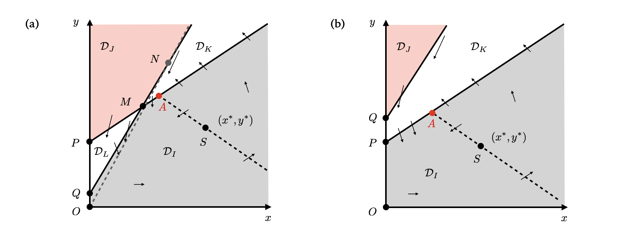
\(O\) is the original point. \(S\) is the positive fixed point. Line \(W^{xx}x-W^{xy}y+u = 0\) intersects \(y\)-axis at point \(P\), and line \(W^{xy}x-W^{yy}y+v = 0\) intersects \(y\)-axis at point \(Q\). \(M\) is the intersection of these two lines. Since \(u, v\geq 0\), \(P,Q\) are both on the half-line \(Oy\), and \(|OQ| = \frac{v}{W^{yy}}\), \(|OP|=\frac{u}{W^{xy}}\). When (1) a positive fixed point exists; (2) \(W^{xx}+W^{yy} < 2W^{xy}\); and (3) \(W^{xx} \geq W^{yy}+2\), there are two cases:

• \(|OP| > |OQ|\), illustrated in Figure (a).
• \(|OP| \leq |OQ|\), illustrated in Figure (b). In this case, we need \(|PQ| < \min\left\{\frac{u}{W^{xy}W^{yy}}, \frac{v}{\left(W^{xy}\right)^2}\right\}\) to ensure the positive fixed point \((x^*,y^*)\) exists.

In both cases, there are three adjacent regions \(\mathcal D_{I}\), \(\mathcal D_{K}\), \(\mathcal D_{J}\). In the region \(\mathcal D_{I}\), as we discussed in the linear case (Lemma 1), the velocity field is anticlockwise around the fixed point \(S\). If find all the points in \(\mathcal D_I\) where the velocity is parallel to the line \(PM\):

where \(k\in \mathbb R\), they all lie on a line

going through the fixed point \(S\).

Now we argue that this line intersect with line \(PM\) at point \(A\), which always lies on the boundary between \(\mathcal D_I\) and \(\mathcal D_K\).

Since \(\dot{x} = -x\) at any points on line \(PM\), including point \(A\), then \(\dot{y}_{A}\) at \(A\) should be \(-x_{A}\cdot W^{xx}/W^{xy}\). Solving

we get the coordinates of \(A\) is \(\left(\frac{W^{yy}u-W^{xy}v+u}{\left(W^{xy}\right)^2-W^{xx}W^{yy}}, \frac{W^{xy}u-W^{xx}v+W^{xx}/W^{xy}\cdot u}{\left(W^{xy}\right)^2-W^{xx}W^{yy}}\right)\). In case (a), the \(y\)-coordinate of \(M\) is \(\frac{W^{xy}u-W^{xx}v}{\left(W^{xy}\right)^2-W^{xx}W^{yy}}\), which is smaller than \(\frac{W^{xy}u-W^{xx}v+W^{xx}/W^{xy}\cdot u}{\left(W^{xy}\right)^2-W^{xx}W^{yy}}\) when \(u > 0\) holds. Since the positive fixed point exists and \(W^{xx}+W^{yy} < 2W^{xy}\), we can verify \(u>0\) must hold. Therefore, point \(A\) is above \(M\) on the line \(PM\). \(A\) is always on the boundary between \(D_I\) and \(D_K\).

In case (b), the \(x\)-coordinate of \(A\) is always positive because

and \(\left(W^{xy}\right)^2-W^{xx}W^{yy} > \left(W^{xx}+W^{yy}\right)^2/4-W^{xx}W^{yy}>0\). Hence, point \(A\) is above \(P\) and always on the boundary between \(D_I\) and \(D_K\). Point \(A\) splits the boundary between \(D_I\) and \(D_K\) into two parts: on the line segment \(MA\) (or \(PA\) in case (b)), the vertical velocity \(\dot{y} < -x\cdot W^{xx}/W^{xy}\); on the half-line above point \(A\), the vertical velocity \(\dot{y} > -x\cdot W^{xx}/W^{xy}\). In other words, trajectories always come into region \(\mathcal D_{I}\) through the line segment \(MA\), (or \(PA\)), and come out from region \(\mathcal D_{I}\) to region \(D_{K}\) through the half-line above point \(A\).

Now we verify the following four claims:

[C1] Every trajectory comes in the region \(\mathcal D_I\) through line segment \(MA\) will come out from the half-line above point \(A\) into region \(\mathcal D_K\).
[C2] Every trajectory in the region \(\mathcal D_K\) will go through line segment \(MA\) into region \(\mathcal D_I\).
[C3] Every trajectory in the region \(\mathcal D_L\) will go through \(\mathcal D_I\) and finally in \(\mathcal D_K\).
[C4] Every trajectory in the region \(\mathcal D_J\) will finally go into \(\mathcal D_K\) or \(\mathcal D_L\).

If a trajectory comes across \(MA\) into \(\mathcal D_I\) (no matter from \(\mathcal D_J\) or \(\mathcal D_K\)), it has two fates: either staying in \(\mathcal D_I\) or leave from somewhere. As we know that the velocity field in \(\mathcal D_I\) is identical to that of the linear network of cases 1(a) and 1(b), this trajectory cannot stay in \(\mathcal D_J\) forever. If it is case 1(a), this trajectory is a part of the arm of an unstable spiral and will go out \(\mathcal D_I\) finally; if it is case 1(b), this trajectory has to be a closed circle in \(\mathcal D_I\), contradicting with the fact that it comes into \(\mathcal D_I\) through \(MA\). Thus, this trajectory has to leave from somewhere. But where?

In the case illustrated in figure (b), the only possibility is half-line above \(A\) on the boundary between \(\mathcal D_I\) and \(\mathcal D_K\). In figure (a) case, we show that it cannot be line segment \(QM\) (the boundary between \(\mathcal D_I\) and \(\mathcal D_L\)). The vertical velocity at points on \(QM\) is always \(\dot{y}=-y\). When discussing the horizontal velocity, line \(PM\) is a good auxiliary. On the line \(PM\), the horizontal velocity \(\dot{x}=-x\). For region below line \(PM\), the horizontal velocity \(\dot{x} > -x\). Therefore, at point \(M\), the velocity is exactly \((\dot{x}_{M},\dot{y}_{M}) = (-x_{M},-y_{M})\), pointing towards \(O\), which is pointing the interior of \(\mathcal D_I\) or along the boundary \(\partial \mathcal D_I\) when \(v=0\). Moreover, the velocities at other points on \(PM\) are all pointing interior \(\mathcal D_I\), as they all have greater horizontal component towards \(x+\). It means in figure (a) case, and trajectories cannot go out \(D_I\) through \(QM\). Hence, our first claim is true.

The trajectories in region \(\mathcal D_{K}\) all have horizontal velocity \(\dot{x} = -x\). In the long term, they have \(x\rightarrow 0\). It indicates they cannot stay in \(\mathcal D_{K}\) forever. In figure (a) case, it asks for trajectories to exceed point \(M\) in the horizontal direction, whose \(x\)-coordinate is non-zero constant as \(u > 0\) must hold. Then they are no longer in the region \(\mathcal D_{K}\). It is a contradiction. Similarly, in figure (b) case, trajectories approch infinitly close to the line segment \(PQ\). But we know that when close to line \(PQ\) the vertical velocity \(\dot{y} \leq \dot{y}_P = v-\left(W^{yy}+1\right)y_P + \epsilon < 0\) for \(v > 0\) (it must hold in figure (b) case otherwise \(u=0\) and no positive fixed point exists.) and any sufficient small \(\epsilon > 0\). It derives \(\int_{0}^{\infty} \dot{y}dt \leq \int_{0}^{\infty} \dot{y}_P dt = -\infty\), the trajectories will exceed point \(P\) in the vertical direction. It leads a contradiction. Then we know that all the trajectories in \(\mathcal D_k\) leave this region from somewhere.

There is actually only one option for those \(\mathcal D_K\) trajectories to go. Since the velocity at any point on the boundary between \(\mathcal D_{K}\) and \(\mathcal D_{J}\) is pointing original point \(O\), when \(|OQ| > 0\), it is always from \(\mathcal D_{J}\) to \(\mathcal {D}_K\); when \(|OQ|=0\), it is along the line \(QM\) and moving towards point \(M\). The velocity at the point \(M\) and on the line segment \(QM\) has been discussed above. Thus, all \(\mathcal D_K\) trajectories all finally go across \(MA\) into \(\mathcal D_I\). The second claim is valid. The last two claims are relatively easier to verify. \(\mathcal D_L\) does not contain fixed point so that \(\mathcal D_L\) goes through \(QM\) into \(\mathcal D_{I}\). Then following the similar argument we made for the first claim, these trajectories will come out \(\mathcal D_I\) the half-line above point \(A\) into region \(\mathcal D_K\), proving the third claim. The velocity in region \(\mathcal D_J\) is \((\dot{x},\dot{y})=(-x,-y)\). If the trajectories are confined in \(\mathcal D_J\), then \(x,y\rightarrow 0\) as time goes to infinite which leads a contradiction since \(y_{P} > 0\). Thus the \(\mathcal D_J\) trajectories will go into \(\mathcal D_L\), \(\mathcal D_K\), or through the point \(M\) into \(\mathcal D_I\) then go to \(\mathcal D_K\). The fourth claim holds.

So far, we make it clear that any trajectory in the plane, either is a closed orbit in the region \(\mathcal D_I\), or eventually shuttles in and out at the boundary between \(\mathcal D_I\) and \(\mathcal D_K\). It is the time to give our proof a final hit — there must exist a stable limit cycle!

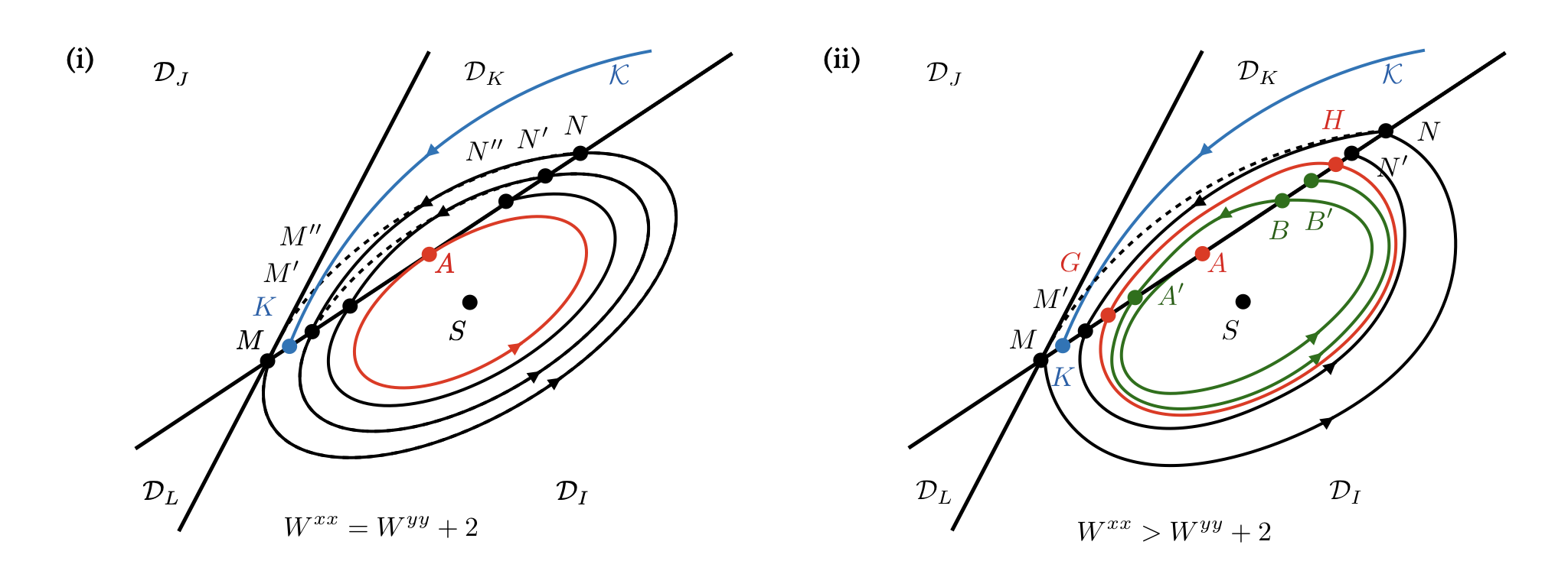
Case i. When \(W^{xx} = W^{yy}+2\), there is a closed trajectory in \(\mathcal D_I\) which tangentially intersects with line \(MA\) at point \(A\). We argue this closed circle is the limit cycle. In the trajectories inner this circle are all closed circles around the fixed point \(S\). Now we show that the outer trajectories spiral into it as time approaches infinity. Consider the trajectory comes into \(\mathcal D_I\) at point \(M\). According to Claim C1, this trajectory will come out \(\mathcal D_I\) at some point \(N\) on the half-line above \(A\) on the boundary between \(\mathcal D_I\) and \(\mathcal D_K\). By Claim C4, it will come back to \(\mathcal D_I\) again through some point on the line segment \(MA\) (or \(PA\) if it is in figure (b) situation. The discussion for these two situations are essentially the same so let us focus on the figure (a) situation, as illustrated above). It cannot go through the endpoint \(M\) again to make itself closed, otherwise another trajectory \(\mathcal K\) in \(\mathcal D_K\) has to intersect with it to be in \(\mathcal D_I\) through \(K\) on \(MA\), which violates the existence and uniqueness theorem. Thus, it revisits \(\mathcal D_I\) through another point \(M'\) on line segment \(MA\), \(|M'M|>0\). Then, it comes to \(\mathcal D_K\) through point \(N'\) on the open line segment \(AN\), and goes back to \(\mathcal D_I\) through the point \(M''\) on the open line segment \(M'A\). Actually, if a trajectory enters \(\mathcal D_I\) at point \(K\) on line segment \(MA\), the next time it will reenter \(\mathcal D_I\) at \(K'\) on the open line segment \(K'A\) if \(K\neq A\). It can be easily verified by calculating the analytical solution of the coordinates of point \(K'\). An intuitive explanation is without nonnegativity constaint, the trajectory will go back to \(K\), but now region \(\mathcal D_K\) sets a “speed limit” for the horizontal velocity but remains the vertical velocity the same. It is like when we throw a ball on a hill, it falls closer when there is horizontal air drag. Therefore, all the trajectories will spiral into the tangent closed circle. It is a stable limit cycle!

Case ii. When \(W^{xx} > W^{yy}+2\), there is an unstable spiral trajectory in \(\mathcal D_I\) which tangentially intersects with line \(MA\) at the point \(A\) and goes to \(\mathcal D_K\) at the point \(B\). This trajectory reenters \(\mathcal D_I\) through point \(A'\) on the line segment \(MA\) by Claim C2 (\(A'\) can be \(A\)), and then exits through point \(B'\) with \(|B'A|\geq |BA|\). If \(A' \neq A\), this suggests there exists an open line segment \(GA\) on line segment \(MA\) such that any trajectory enters \(\mathcal D_I\) through some point \(K\) on \(GA\) (\(K\neq G\)), will reenter \(\mathcal D_I\) through some point \(K'\) on the open line segment \(GK\). Also, there exists an open line segment \(AH\) on the half-line above \(A\) such that any trajectory leaves \(\mathcal D_I\) through some point \(K\)(\(K\neq H\)) on \(AH\), will leave \(\mathcal D_I\) next time through some point \(K'\) on the open line segment \(KH\). However, if we investigate trajectory coming into \(\mathcal D_I\) through point \(M\), following the same argument we have made in case i, it will spiral inward. Thus, it suggests any trajectory enters \(\mathcal D_I\) through some point \(K\) (\(K\neq G\)) on \(MG\), will reenter \(\mathcal D_I\) through some point \(K'\) on the open line segment \(KG\). Also, any trajectory leaves \(\mathcal D_I\) through some point \(K\) (\(K\neq H\)), will leave \(\mathcal D_I\) next time through some point \(K'\) on the open line segment \(HK\). All these arguments can be verified by calculating coordinates of \(K'\) given \(K\). If there is a trajectory passes through \(G\) then it will pass \(H\), and revisit \(G\) again. Otherwise, it will intersect with adjacent orbits. This has to be a closed orbit. Therefore, all the trajectories spiral to approach a closed orbit going through \(G\) and \(H\) as time go to infinity!

To sum up, when (1) a positive fixed point exists; (2) \(W^{xx}+W^{yy} < 2W_{xy}\); and (3) \(W^{xx} \geq W^{yy}+2\), there is a stable limit cycle in \(\mathcal D_I\) if \(\tau =0\), and a limit cycle across \(\mathcal D_I\) and \(D_K\) if \(\tau > 0\). Combined with the necessity arguments, these three conditions are necessary and sufficient for the existence of limit cycle.

Q.E.D.

CASE 3: Time Constants (n=r=1)

We add two time constants \(\tau_x > 0\) and \(\tau_y > 0\) to contral the speed of excitatory and inhibitory synapses. The dynamics of the neural network is defined by

where \(W^{xx}, W^{xy}, W^{yy} > 0\), \(x, y, u, v \geq 0\), and \(W^{xy} = W^{yx}\). Adding times constants does not change the division of regions \(\mathcal D_I\), \(\mathcal D_J\), \(\mathcal D_K\), and \(\mathcal D_L\). Also, it does not change the existence and the location of positive fixed point \((x^*,y^*)\). It will change the trace and the determinant of Jacobian

respectively. The discriminant becomes

We update Theorem 2 to include the time constants: in a rectified linear neural network, a limit cycle exists if and only if all the following conditions hold:

  (1) a positive fixed point exists;
  (2) \({\bf \sqrt{\tau_y/\tau_x}\left(W^{xx}-1\right)+\sqrt{\tau_x/\tau_y}\left(W^{yy}+1\right) < 2W^{xy}}\); and
  (3) \({\bf (W^{xx}-1)/\tau_x\geq (W^{yy}+1)/\tau_y}\).

When the inhibition is much faster than the excitation, i.e., \(\tau_y/\tau_x \rightarrow 0\), it is impossible to produce limit cycles in an E-I network.

Author & Copyright

Runzhe Yang
Please contact the author to cite this work.