How Many Memories Can We Recall?

Memory cannot be understood, either, without a mathematical approach. The fundamental given is the ratio between the amount of time in the lived life and the amount of time from that life that is stored in memory. No one has ever tried to calculate this ratio, and in fact there exists no technique for doing so; yet without much risk of error I could assume that the memory retains no more than a millionth, a hundred-millionth, in short an utterly infinitesimal bit of the lived life. That fact too is part of the essence of man. If someone could retain in his memory everything he had experienced, if he could at any time call up any fragment of his past, he would be nothing like human beings: neither his loves nor his friendships nor his angers nor his capacity to forgive or avenge would resemble ours.

— Milan Kundera, Ignorance (2000)

Human memory is fragile. We’ve probably already forgotten what we ate last Christmas Eve, let alone those complicated equations of reactions that we learned long ago in Chemistry classes. A couple lasting for years can struggle to remember the passion ignited at the beginning of their love story. Does all this mean that we should blame the long and tedious passage of time for our poor memory? If so, how do we find an excuse for the unfortunate man who is now in the supermarket and once again forgets to bring his family’s grocery list? His challenge is to recall as many items as possible to buy before driving back home with missing items. If he fails, he will have to face an upset wife upon his return. The unreliable memory, as a charmingly annoying defect of mankind, is responsible for so much forgetting and forgiveness in everyday trivialities, and likely accounts for countless regressions and recurrences throughout history.

Scientists still know so little about our memory. There are different types, such as sensory, short-term, and long-term memory, and many aspects, including formation, storage, and retrieval, that one can wonder about. However, most of them remain shrouded in a thick fog of ignorance. A widely accepted postulate is that the learning process changes the weights of synaptic connections among neurons in the brain, and these modified connections may encode our memories (Kandel, 2001). At the molecular and cellular level, researchers are still searching for the related biochemical mechanisms of synaptic plasticity, which is akin to solving a giant jigsaw puzzle with many pieces yet to be found (Kern et al., 2015; Harward et al., 2016; Ford et al., 2019). At the level of neural systems, many elegant models and theories have been proposed (Hopfield, 1982; Seung, 1996; Goldman, 2009), but testing them with biological evidence has not been easy (connectomics is bringing some hope). At the behavioral and cognitive level, human memory properties exhibit extreme variability across different experimental conditions (Waugh, 1967; Standing, 1973; Howard and Kahana, 1999), making it challenging to acquire quantitative descriptions.

No wonder Kundera complained in his novel about the limited knowledge of memory, particularly the absence of a good mathematical understanding. One ultimate challenge in the study of memory is to derive law-like principles that can match the precision and generality of Newton’s laws. Is this possible? I believe that today’s psychology and neuroscience offer the most promising prospects for an affirmative answer. At the very least, there are scientific narratives, both old and recent, that would undoubtedly bring delight to both a sympathetic novelist and a forgetful husband.

• Kundera’s ratio
  • Standing’s scaling law
  • Recognition and free recall
• Fundamental law of memory recall
  • Associative memory networks
  • Memory transition via oscillatory inhibition
  • Birthday paradox of the recall model

Kundera’s ratio

What Kundera argued to be important, was the ratio between the number of items retained in memory (\(M\)) and the number of items presented (\(S\)). Here, I covertly convert his measurement of continuous time to the counts of discrete items for simplification. He suspected that this ratio was infinitesimal for a lived life. Was he correct?

Intuitively, we can quickly check based on our own experience. Childhood was the heyday of our memory. Children observe the world carefully and seem to remember almost everything that happens in their surroundings. The patterns on sheets, the names of toys, the stories told by grandpa after last Saturday’s dinner—none of them are too difficult for a child to recall. Therefore, Kundera’s ratio is conceivably high for children, not only because they are curious observers of the world but also because they are just starting to learn things, resulting in a small denominator for the ratio. However, as we grow up, we perceive a more complex world, and soon the total number of things presented (\(S\)) far surpasses the total number of things we remember (\(M\)). The ratio proposed by Kundera is less likely to be a constant but rather decreases rapidly as life progresses. The retained memory increases sublinearly in relation to the things presented, so the ratio indeed becomes small over our normal lifespan.

Kundera claimed that no one had ever attempted to calculate this ratio, and there was no technique like telepathy available. However, in the 1960s, some efforts were made to calculate this ratio for short-term memory by Nickerson (1965) and Shepard (1967), and extended to long-term memory by Nickerson (1968). In Nickerson’s study, subjects were shown 612 pictures and then asked to select the correct pictures in two-alternative recognition tests. The accuracy was remarkably high at 98%. These results appear to contradict Kundera’s speculation. However, sublinear retention growth is supported by an influential study conducted by (Standing, 1973). Kundera might have missed these interesting studies in 2000, as Google Scholar had not yet been invented.

Standing’s scaling law

In a 1973 study, Lionel Standing conducted a delayed recognition task to estimate the capacity of our long-term memory. Participants were divided into groups and exposed to various sets of stimuli during a single-trial learning phase, with strict concentration. These stimuli were selected from a pool consisting of 11,000 normal pictures, 1,200 vivid pictures, and 25,000 of the most common English words from the Merriam-Webster dictionary. Two days later, the participants took part in a recognition test. In each trial, two stimuli were presented side by side, with only one stimulus being correct and from the learning sets, while the other was randomly chosen from the remaining stimuli in the entire set. The participants were required to indicate their familiarity by writing down an “L” or “R” to indicate which stimulus they found more familiar. The estimated number of items in memory (\(M\)) was then calculated as follows:

where \(E\) is the number of errors, \(T\) is the total number of trials, and \(S\) is the size of the learning set. What is the rationale behind this calculation? If the correct stimulus is present in a subject’s memory, they would answer correctly. However, if the correct stimulus is not in a subject’s memory, they would randomly choose one, resulting in an error rate of 0.5. Therefore, the total error rate can be calculated as follows:

Rearranging the above equation gives the estimate of \(M\).

With the experimental data, Standing observed that memory for pictures (◾ and ◯) was superior to memory for verbal information (▼). For instance, when the size of the learning set was 1,000, the accuracy for word recognition was only 62%, while it reached 88% for vivid images. Furthermore, there was a power-law relationship between the number of items presented for learning \((S)\) and the number of items retained in memory (\(M\)). The figure below illustrates this relationship, where all three stimulus populations resulted in straight lines when plotting \(\log M\) against \(\log S\), with a Pearson correlation coefficient exceeding 0.99.

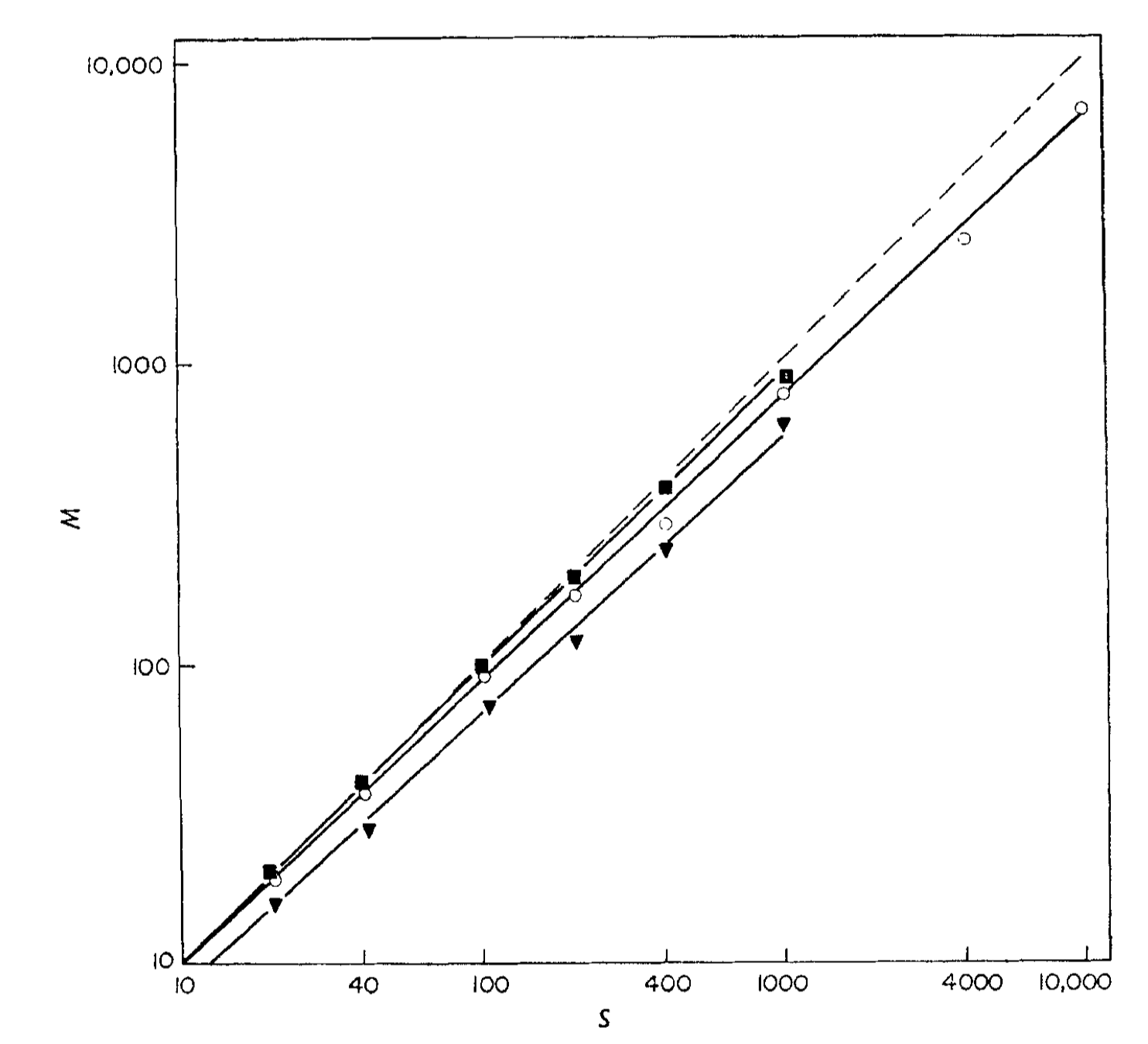Figure 1 in Standing (1973). Number of items retained in memory (\(M\)), as a function of number presented for learning (\(S\)). The diagonal dashed line indicates perfect memory. ◾ vivid pictures (\(\log M \approx 0.97\log S + 0.04\)); ◯ normal pictures (\(\log M\approx 0.93 \log S + 0.08\)); ▼ words (\(\log M \approx 0.92\log S-0.01\)). Note that the coordinates are log-log.

The straight line observed in the log-log plot suggests a general mathematical relationship for retained memory:

where \(a >0, 0 <\beta \leq 1\). The exponent \(\beta\) indicates how quickly the retained memory increases as the number of presented items grows. These exponents correspond to the slopes of the lines in the log-log plot (\(\log M = \beta \log S + \log a\)). When \(\beta=1\), the ratio \(M/S\) remains constant. The \(\beta\) value for normal picture memory was approximately 0.93. This implies that if Kundera’s ratio is less than one millionth, we would need a minimal learning set containing around ~\(10^{86}\) stimuli. However, this seems improbable given that a person living for 100 years only has approximately \(3.2 \times 10^9\) seconds. Using the same \(\beta\) value and assuming: 1) the time scale for memorization is on the order of seconds, and 2) successfully formed memories are not erased, the estimated Kundera’s ratio for a 100-year lifespan would be around 23%. These findings indicate that our brain is far more capable of retaining information in memory than Kundera’s speculative estimation suggests.

Recognition and free recall

Standing’s scaling law raises high expectations for the man who forgot to bring the grocery list to the supermarket. Assuming the list contained 20 items, according to the scaling law, the expected number of items he would retain in his memory should be approximately \(20^{0.92} \approx 16\). However, he feels frustrated and unable to recall any of them. Could we conclude that those memories have been erased? Or is it possible that the memories are still intact, but he simply struggles to retrieve them all?

I suspect it’s the latter case. If the man happens to see the item he intended to buy, he would likely recognize it on the shelf without much contemplation. It’s akin to those embarrassing moments when we suddenly forget the name of a friend, only to have it quickly come to mind when someone mentions it. Recognizing something we should remember is fundamentally different from the cue-less process of recall, and the latter is intuitively more challenging. In a recognition test, a cue is provided to trigger the correct memory. However, in a free recall task, no external hint is given, requiring one to meticulously search within their memory palace to locate the correct answer.

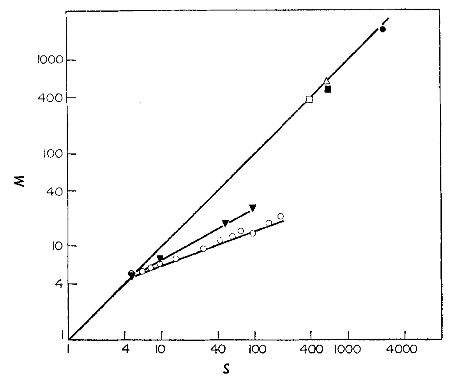Figure 2 in Standing (1973). Number of items retained in memory or successfully recalled (\(M\)), as a function of the number presented for learning (\(S\)). □ Nickerson 1965 (pictures, recognition); △ Shepard 1967 (pictures, recognition) ◾ Shepard 1967 (words, recognition); ▼ Binet and Henri 1894 (words, recall); ◯ Murdock 1960 (words, recall). The coordinates are log-log.

Our observation that recognition performance surpasses recall is substantiated by experimental data. In the above figure, Standing compiled experimental results from free recall tests conducted by Binet and Henri (1894) and Murdock (1960) (represented by the two lines with smaller slopes in the figure), and compared them to previous recognition results. All the data points align along straight lines in the log-log plot, with a Pearson correlation coefficient exceeding 0.99. This indicates that the power law holds true for both recognition and recall. The number of items successfully recalled \((R)\) can be expressed as

where \(c >0, 0 <\gamma \leq 1\). Notably, the exponent \(\gamma\) for recall is lower than the exponent \(\beta\) for actual retained memory, as estimated by recognition tests. This suggests that sometimes we struggle to remember things not because we have forgotten them entirely, but because we encounter difficulties in recalling the information retained in memory. Another significant deduction is that the number of recalled items also follows a power function in relation to the number of items retained in memory.

Despite our effective ability to store things in memory, as indicated by a value of \(\beta \approx 0.93\), if the retrieval process is inefficient, with \(\theta \approx 0.5\) for instance, the ratio between the number of items we can recall and the number of items we have experienced will rapidly decrease to less than a millionth within a 100-year lifespan. This outcome supports Kundera’s conjecture—although we can retain many memories, we can only recall a small fraction of them. As forgetful humans, we rely on someone or something to remind us.

Fundamental law of memory recall

There are several classic theoretical models that can effectively explain the empirical data for memory retrieval. One such theory is the probabilistic search of associative memory (SAM) model (Raaijmakers and Shiffrin, 1980; 1981). SAM assumes that all presented stimuli are stored in memory buffers, and the recall process is modeled as a series of probabilistic attempts to sample memory items until a certain number of failed attempts is reached. Another influential theory is the temporal context model (TCM) (Howard and Kahana, 2002; Polyn, Norman, & Kahana, 2009). TCM considers time-dependent context to replicate the effects of end-of-list recency and lag-recency in free recall (Murdock, 1962; Kahana, 1996). However, these models involve numerous parameters that need to be fine-tuned for each learning set size (\(S\)) and are too complex to reveal the fundamental neural network mechanism of memory retrieval (Grossberg and Pearson, 2008).

In recent years, a series of studies by Sandro Romani, Mikhail Katkov, Misha Tsodyks, and their collaborators (Romani et al., 2013; Recanatesi, 2015; Katkov et al., 2017; Naim et al., 2020) propose a simple neural network model for memory recall. This model exhibits a scaling law similar to that observed by Standing (1973) but without the need for free parameters. According to their theory, there exists a fundamental relationship between the number of recalled items (\(R\)) and the number of items retained in memory (\(M\)), which can be expressed as follows:

This remarkably simple formula, derived purely from mathematical deduction, astonishingly aligns with the experimental data. In Naim et al. (2020), the researchers estimated \(M\) from the recognition tasks and \(R\) from the free recall tasks, similar to the approach employed by Standing (1973). The stimuli used in their experiments consisted of a collection of 751 English words and 325 short sentences expressing common knowledge facts (e.g., “Earth is round”). Notably, all the experimental data strongly support the theoretical predictions.

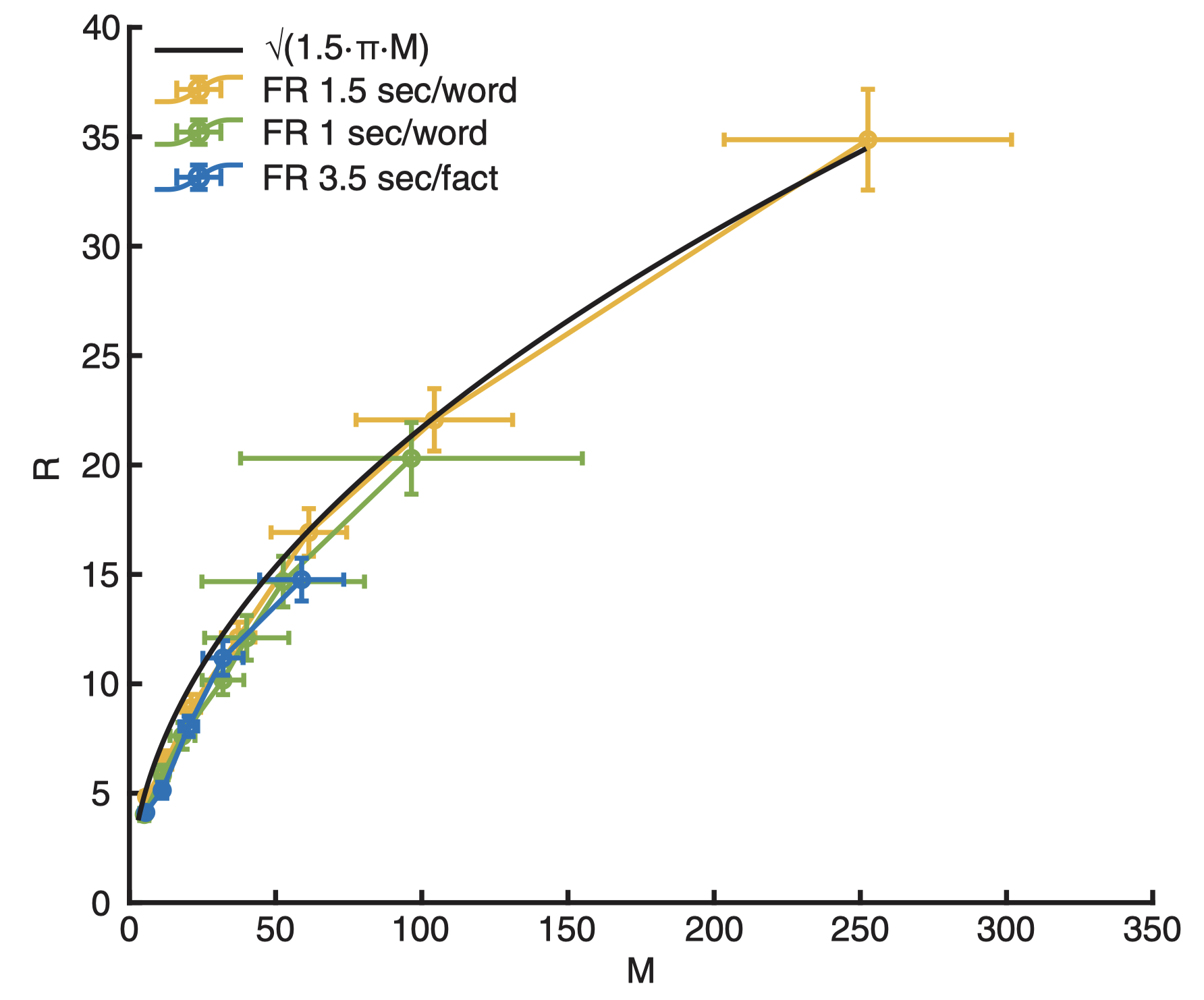Figure 2 in Naim et al. (2020). The average number of words (sentences) recalled as a function of the average number of words (sentences) retained in memory. Black line: Theoretical prediction (\(R =\sqrt{3\pi M/2}\)). Green line: experimental results for presentation rate 1 word/sec. Yellow line: experimental results for presentation rate 1.5 word/sec. Blue line: experimental results for short sentences of common knowledge facts.

The theory not only generates the scaling law that psychologists have empirically summarized but also provides insights into the parameters of the scaling law. Where does the peculiar constant \(d = \sqrt{3\pi/2} \approx 2.17\) originate? And how do we interpret the exponent \(\theta = 0.5\)? In the remaining sections of this article, we will delve into the mathematical details to gain a deeper understanding.

Associative memory networks

The proposed theory is grounded in two fundamental principles (Katkov, Romani, & Tsodyks, 2017):

• [Encoding Principle] - An item is encoded in the brain by a specific group of neurons in a dedicated memory network. When an item is recalled, either spontaneously or when triggered by an external cue, this specific group of neurons is activated.
• [Associativity Principle] - In the absence of sensory cues, a retrieved item plays the role of an internal cue that triggers the retrieval of the next item.

The first encoding principle can be realized by the classic associative memory networks (Hopfield, 1982), where the items retained in memory are encoded through binary activity patterns of \(N\) neurons within a specific network. For example:

where “1” indicates an active neuron, and “0” indicates a inactive neuron. The neurons within the network are interconnected in a specific manner such that when only a subset of neurons is activated by an external cue, even with noise, the network activity will converge to the most similar stored memory. These stored memories are also referred to as attractors of the neural networks.

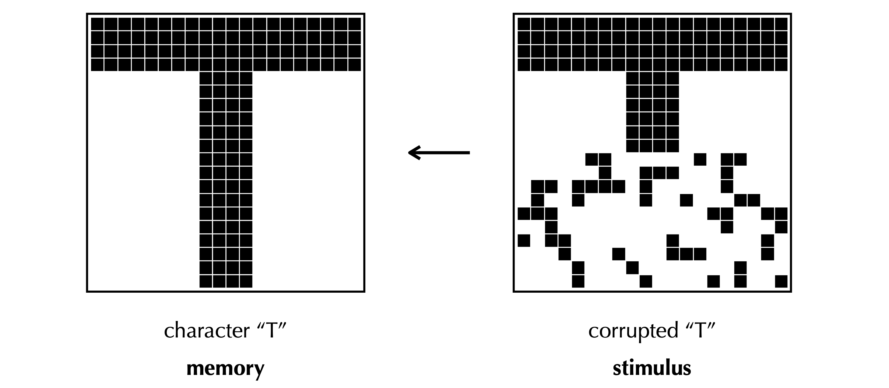An illustration of memory retrieval from my slides. An image “T” encoded by binary neural activity is stored in an associative memory model. Each pixel here indicates a neuron. When the external cue, a corrupted “T”, is given, the network is able to restore the correct image. See my slides to quickly recap the classic idea of Hopfield nets. The slides also introduce recent advances (Krotov and Hopfield, 2016; Krotov and Hopfield, 2020) to increase the memory capacity of Hopfield nets from \(\mathcal O(N)\) to \(\mathcal O(e^N)\).

The original Hopfield networks were capable of reliably storing multiple uncorrelated random memories, where approximately half of the neurons would be active for each stored memory. However, neurophysiological data suggest that neural activity is typically sparse, meaning that the percentage of active neurons for each memory, denoted as \(f\), is very small. In such cases, the synaptic connectivity needs to be modified as follows (Tsodyks & Feigel’Man, 1988):

with a special condition where \(T_{ii} = 0\). Here, \(T_{ij}\) represents the connection strength from neuron \(j\) to neuron \(i\), \(M\) is the total number of items retained in memory, and \(N\) is the total number of neurons. When \(f \ll 1\), neuron \(i\) and neuron \(j\) exhibit strong connections when they are both active within a single memory. Consequently, if we focus only on the strong connections within an associative memory network, the stored memories form \(M\) potentially overlapping cliques.

The dynamics of neural activity, denoted as \(\sigma_i(t)\in \{0, 1\}\) can be described by the following equation (Romani et al., 2013)

where \(\Theta(\cdot)\) is the Heaviside function, \(J>0\) represents the strength of global feedback inhibition that controls the overall level of activity, and \(\theta_i(t) \in [-\kappa, \kappa]\) denotes the threshold for the neuron \(i\).

Consider the energy function:

where the first quadratic term involves the dot product of the memory \(\boldsymbol \xi^{\mu}-f\) and the current neural activity \(\boldsymbol \sigma\). The second and third terms are prominent when \(\boldsymbol \sigma\) is dense. The dynamics of neural activity can be interpreted as monotonically minimizing the energy function because when the activity of neuron \(i\) changes by \(\Delta \sigma_i\), the change in energy can be expressed as:

\(\Delta H < 0\) if and only if \(\Delta \sigma_i\) has the same sign as \(\sum_{j=1}^{N}T_{ij}\sigma_j - \frac{J}{Nf} \sum_{j=1}^N\sigma_j- \theta_i\), which is always guaranteed by the neural activity dynamics. Hence, the local minima of \(H(\boldsymbol \sigma)\) correspond to steady activities. When \(\boldsymbol \sigma(t)\) is dense, the global inhibition is strong, leading to the suppression of many neurons to encourage sparsity. When the number of memories \(M\) is below a certain capacity limit (where memories \(\boldsymbol \xi^{\mu\in\{1,\dots,M\}}\) are less likely to “interfere” with each other), with a specific small \(J\) and \(\theta_i\), we can deduce from the expression of the energy function that the steady activity corresponds to one of the stored memories, i.e., \(\sigma_i = \xi^{\mu}_i\), which minimizes the first quadratic term of \(H\) while satisfying the sparsity constraints. In other words, under specific conditions of global inhibition strength \(J\) and threshold \(\theta_i\) for each neuron, a memory can be stably retrieved by a similar external cue.

Memory transition via oscillatory inhibition

In the absence of an external cue, how can we recall information from the associative memory network? Intuitively, if two memories are similar, we should be able to establish an association between them. This idea corresponds to the second associativity principle. The proposal put forward by Romani et al. (2013) is to create a steady neural activity pattern that alternates between stored memory representations and the intersection of two memory representations. This allows for a smooth transition of the mental state from one attractor to another without requiring an external cue.

The strength of the global feedback inhibition, denoted as \(J\), plays a crucial role in controlling the steady neural activity. As mentioned earlier, for small values of \(J\), the memory representations remain stable. However, as \(J\) is increased, more neurons are inhibited, guiding the neural activity towards the intersection of two memory representations. This process facilitates the transition between different memories in the absence of external cues.

When the number of neurons, denoted as \(N\), is large and memory representations are sparse (\(\xi_i^{\mu} \sim \text{Bernoulli}(f)\) independently for all \(i\) and \(\mu\), where \(f \ll 1\)), we can utilize the law of large numbers to make approximations. Specifically, we have:

To determine the conditions for stable memory representations, we can set the initial activity as a memory \(\boldsymbol \xi^{\mu}\). By employing the aforementioned statistics, we obtain self-consistent equations for all \(i\):

Since \(\theta_i \in [-\kappa, \kappa]\), solving the above equation yields \(J\in (\kappa - f, 1-\kappa-f)\).

Similarly, to derive the conditions for stable overlaps between two memory representations, we initialize the neural activity with \(\boldsymbol \sigma(0) = \boldsymbol \xi^{\mu} \odot \boldsymbol \xi^{\nu}\), where “\(\odot\)” denotes the element-wise product. This results in a set of self-consistent equations:

Thus, when \(J\in (1 - 2f + \kappa/f, 2-2f-\kappa/f)\), the overlap of two memories remains stable.

Figure 1 in Romani et al. (2013). (A) Dynamics of a network storing 16 items with periodically oscillatory inhibition and threshold adaptation. (B) The matrix of overlaps between memory representations.

Simulations have demonstrated that periodically oscillating \(J\) between these two regimes can effectively produce a sequence of recalled items in memory. To avoid the neural activity from reverting back to the memory that was just recalled, thresholds \(\theta_i(t)\) adapt in an activity-dependent manner. In the simulations, when an item is recalled, it often triggers the subsequent retrieval of an item that shares the largest overlap in memory representation. This phenomenon can be interpreted as the recall process involving a sequence of associations among similar memories, providing us with an intriguing mathematical understanding of the limitations of our memory recall capabilities.

Birthday paradox of the recall model

The recall process, implemented by the neural network model described above with periodic modulation of inhibition, can be further abstracted and simplified as a walk among stored memories. The mental state transitions from one memory to another based on the degree of neuron activation overlap. If the most similar memory has just been recalled, the mental state moves to the memory with the second-largest overlap in activation.

The similarity score, or relative size of memory overlap, between two different memories \(\mu\) and \(\nu\), is quantified by the dot product of their binary neuronal representations normalized by the total number of neurons:

The similarity scores form a symmetric matrix of size \(M \times M\) for any two distinct memories, where we set all diagonal elements \(s^{\mu \mu} := 0\) for convenience. While the similarities are symmetric, it is worth noting that the “most similar” relationship induced by these scores may not be symmetric. This is similar to the disheartening fact that you have only a 1/2 chance of being the best friend of your best friend, even though the friendship is mutual. This probability can be justified by:

where \(s^{\mu \nu} = s^{\nu \mu}\) and the number of friends (\(M\)) is large. Additionally, we assume a large \(N\) so that the similarity scores \(s^{\mu \nu}\) can be treated as continuous values, ensuring that the chance of two pairs of items having the same similarity score is almost zero.

The asymmetric “most similar” relationship creates a directed pathway that connects different items in memory. This allows for transitions from item \(\mu\) to item \(\arg\max_\omega s^{\mu\omega}\), enabling the traversal of multiple items in a chain. For example, in the similarity matrix shown below, item 13 has item 1 as its most similar item, while item 1 has item 14 as its most similar item. Therefore, the sequence 13 → 1 → 14 represents a chain of recalled items.

However, as we discussed earlier, at each step, there is a 1/2 chance of returning to the previously recalled item, potentially leading to a two-item cycle and limiting the number of recalled items to three, no matter how many items are stored (note that here the randomness comes from the similarity matrix, when assuming a large \(N\), but transitions are deterministic).

To address this issue, we need a modification that allows the recall process to move to the “second most similar” item when the most similar one has been visited in the previous immediate step. This modification results in longer paths that involve a greater number of items. The recall process terminates when it starts cycling over already visited items.

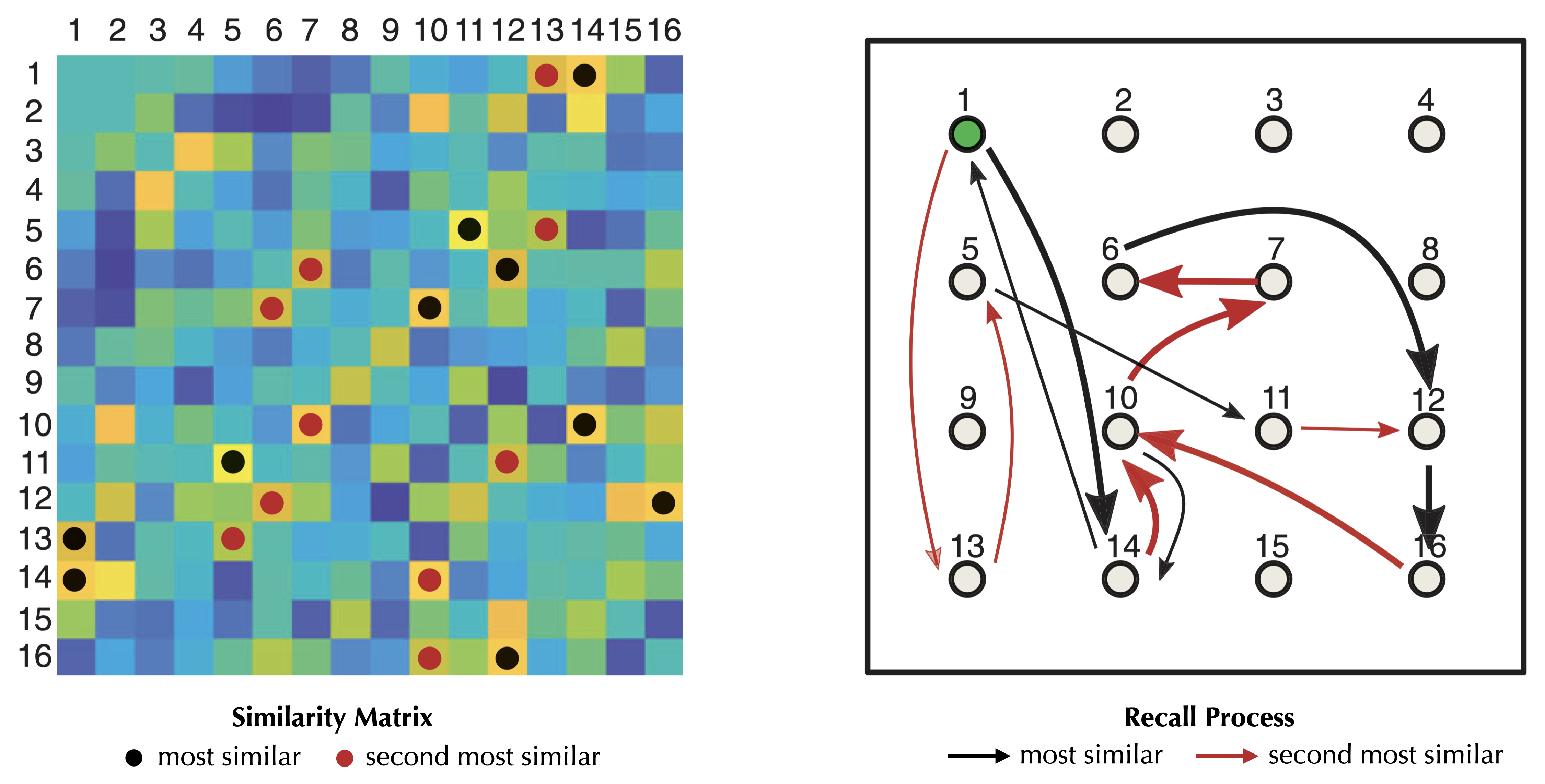Modified from Figure 1 in Naim et al. (2020). Left: a symmetric similarity matrix among 16 items retained in memory. Warmer color indicate a higher similarity score. Black circles and red circles indicate the highest and the second highest similarity scores in each row, respectively. Right: the recall process as a deterministic walk among items stored in memory. Black arrows indicate moving to the most similar item, and red arrows indicate moving to the second most similar item when the memory of the current item is just triggered by its most similar one. The recall path starting from the item 1: 1 → 14 → 10 → 7 → 6 → 12 → 16 → 10 → 14 → 1 → 13 → 5 → 11 → 12 → 16 … (cycle).

How many unique items can be retrieved in such a recall process? Each time we return to a previously recalled item \(\mu\) from a newly recalled item \(\nu\), the next item to be retrieved is considered new only if \(\mu\) is the initial item, and has not been visited through transitions from other items. This is because if \(\mu\) is not the initial item or has already been retrieved in a previous transition, such as \(u\) → \(\mu\) → \(w\), with \(u \neq \nu\), then either (a) \(s^{\mu w}\) is the maximum in the row \(s^{\mu \cdot}\), or (b) \(s^{\mu u}\) is the largest and \(s^{\mu w}\) is the second largest elements in the row \(s^{\mu \cdot}\). As a result, there are only two possible scenarios for the subsequent retrieval after revisiting such an item \(\mu\):

1. Repeating a past transition between two previously recalled items (\(\mu\) → \(w\) → …, if condition (a) holds), which leads to a loop in the recall process.
2. Traveling backward along a novel transition to the already visited items (\(\mu\) → \(u\) → …, if condition (b) holds) until encountering a new item, or reaching a loop.

Case 1 indicates the termination of the recall process, as illustrated by the transition 11 → 12 in the example pathway. Case 2, on the other hand, allows for the continuation of the recall process, as exemplified by the transitions 16 → 10 → 14 → 1 → 13.

Case 2 can occur multiple times in a recall process, and only at its first occurrence, it is guaranteed to lead to a new trajectory since it can return to the initial item and embark on a new route. However, but this does not garuantee new itmes, since the second similar item to the initial item could be visited. More over, if case 2 happens multiple times, it must result in a loop since the the alternative pathways have been exhausted (e.g., if we change the transition 13 → 5 to 13 → 7 in the example pathway and similarity matrix, it is again the case 2 but ends up with a loop.). These particular scenarios require further discussion and investigation, which is not explicitly addressed in Naim et al. (2020). In order to replicate their theoretical findings, it is assumed that when \(M\) is sufficiently large, the likelihood of encountering a loop in the case 2 is negligible.

Thus, in order to determine the number of unique items recalled, we need to understand the probability, \(p_r\), of returning to an already recalled item \(\mu\) from a newly recalled item \(\nu\), and the probability, \(p_{\ell}\), of encountering case 1 where the subsequent retrieval leads to a loop. Analyzing these probabilities is challenging due to the interdependencies among the similarity scores. While Romani et al. (2013) demonstrate that the correlations between similarity scores become negligible in the limit of very sparse memory representation (\(f\ll 1\)), I am unsure about the justification for assuming independence and the validity of their Gaussian approximation, \(s^{\mu\nu} \approx zm_\mu m_\nu\), which preserves the original first- and second-order statistics. In principle, we can compare the joint probability with the product of the two marginal probabilities and demonstrate that, as \(N\) grows, they become asymptotically equivalent when \(Nf\) is a constant. This suggests that, at least in a sparse limit, the similarity scores within each row can be treated as asymptotically independent of one another.

Under the assumption of independence, the probability of revisit, \(p_r\), is calculated as:

Here, for the transition \(\nu\) → \(\mu\) to be possible, \(s^{\mu\nu}\) must be one of the top two values in the row \(s^{\nu\cdot}\) (or equivalently, the column \(s^{\cdot\nu}\)). Additionally, \(s^{\mu\nu}\) must not be the highest value in the row \(s^{\mu\cdot}\), as this would contradict the assumption that \(\nu\) is a newly visited item followed by the transition \(\nu\) → \(\mu\).

For a past trajectory \(u\) → \(\mu\) → \(w\), the probability \(p_{\ell}\) of entering case 1 (\(\mu\) → \(w\), instead of the backward transition \(\mu\) → \(u\)) requires \(s^{\mu u}\) to be a non-maximum value in the row \(s^{\mu \cdot}\), given that the similarity to the newly visited item \(\nu\), \(s^{\mu\nu}\), is also a non-maximum value in the row \(s^{\mu \cdot}\). This leads to the probability:

We derive this probability by considering all three orders of \(\max s^{\mu\cdot}\), \(\max s^{u\cdot}\), and \(\max s^{\nu\cdot}\) with the condition that \(\max s^{\nu\cdot} < \max s^{\mu\cdot}\). Out of these three orders, only 2 out of 3 satisfy the condition \(\max s^{\mu\cdot} > \max s^{u\cdot}\).

Combining these probabilities, the overall probability of returning to a previously recalled item \(\mu\) and terminating the process after each newly retrieved item is:

The recall process is thereby similar to the famous “birthday paradox.” Suppose that we have a group of \(M\) randomly chosen people with uniformly distributed birthdays. We ask them to enter a room one by one, until a pair of people in the room have the same birthday. The probability of two people sharing the same birthday is \(p\). The expected number of people in the room at the end of the process is equivalent to the expected number of unique memories recalled.

The probability that the number of unique items recalled (\(R\)) is greater than or equal to \(k\) can be expressed as:

This approximation holds when \(k \ll M\) and \(1\ll M\). When \(M\) is finite, and \(k\) is large, this probability decays exponentially. Therefore, when considering the expectation under this probability distribution, it is dominated by small \(k\) where the above approximation is valid. The expectation of \(R\) can be asymptotically calculated as

By substituting \(p = 1/(3M)\), we obtain:

Thus, both the exponent (\(\theta = 1/2\)) and the coefficient (\(d=\sqrt{3\pi/2}\) ) of the observed power law are consequences of the “birthday paradox” inherent in the assumed recall process. In this process, the mental state deterministically travels from one memory to its most similar or second most similar memories and eventually ends with a cycle when encountering a previously visited memory.

July 12, 2023: The narrative of the renowned author Milan Kundera has reached its conclusion, yet the enduring battle between memory and forgetting persists.